Some efficient ways to invert a binary tree

Written on August 16, 2022

It is the most famous LeetCode problem of all time, and a task that every FAANG (or MANGA?) software engineer must know by heart: inverting a binary tree. It’s also one that the inventer of Homebrew famously flubbed in a Google interview (and, less famously and more recently, so did I!) In this post I want to take a closer look at this problem and talk about some truly absurd ways you might choose to answer it in an interview. But first, let’s recap the problem.

Problem statement

A binary tree is a directed, simply connected, acyclic graph where each vertex has one incoming edge and (at most) two outgoing edges, and each edge is either a “left” edge or a “right” edge. In addition the vertices of the graph may be decorated with arbitrary values (such as integers or strings). A picture (from LeetCode) is below:

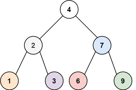
This structure commonly appears in search and sorting algorithms, where the “left” and “right” relationships indicate an ordering among the elements of the graph, and the vertex decorations are the elements of the collection being sorted or searched.

The most basic approach to this problem is to represent the tree as a data structure consisting of the vertex’s value and pointers to the left and right children:

class TreeNode(object):
    def __init__(self, val, left=None, right=None):
        self.val = val
        self.left = left
        self.right = right

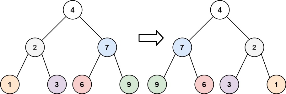
Inverting a binary tree in this context simply means reversing the ordering of the edges, that is, converting every “left” edge to a “right” edge:

The typical interviewer will expect you to write a recursive algorithm to swap the order of the children, for example:

def invert(tree):
    if tree is None:
        return tree
    _left = invert(tree.left)
    _right = invert(tree.right)
    tree.left = _right
    tree.right = _left
    return tree

This approach has to visit each vertex once, and so should have time complexity \(\mathcal{O}(n)\), where $n$ is the number of vertices in the graph.

And this is all fine and dandy, congratulations on your new job at Amazon!

But we can do better…

Vectorizing the tree inversion

Any directed graph can be represented as an adjacency matrix $A$ where $A_{i,j} = 1$ if there is an edge from vertex $i$ to vertex $j$. In the example above, we would have an adjacency matrix:

\[A = \left(\begin{matrix}0 & 0 & 0 & 0 & 0 & 0 & 0\\ 1 & 0 & 1 & 0 & 0 & 0 & 0\\ 0 & 0 & 0 & 0 & 0 & 0 & 0\\ 0 & 1 & 0 & 0 & 0 & 0 & 1\\ 0 & 0 & 0 & 0 & 0 & 0 & 0\\ 0 & 0 & 0 & 0 & 1 & 0 & 1\\ 0 & 0 & 0 & 0 & 0 & 0 & 0 \end{matrix}\right)\]

with vertex decorations (note that there are only 7 vertices)

\[\left(\begin{matrix}1 & 2 & 3 & 4 & 6 & 7 & 9\end{matrix}\right)\]

But how do we encode the “left” and “right” nodes in this setup?

One way to do it is to sign the adjacency matrix: \(A_{ij} = -1\) if the edge from $i$ to $j$ is a left node, and $A_{ij} = 1$ if it’s a right node:

\[\tilde{A} = \left(\begin{matrix}0 & 0 & 0 & 0 & 0 & 0 & 0\\ -1 & 0 & 1 & 0 & 0 & 0 & 0\\ 0 & 0 & 0 & 0 & 0 & 0 & 0\\ 0 & -1 & 0 & 0 & 0 & 0 & 1\\ 0 & 0 & 0 & 0 & 0 & 0 & 0\\ 0 & 0 & 0 & 0 & -1 & 0 & 1\\ 0 & 0 & 0 & 0 & 0 & 0 & 0 \end{matrix}\right)\]

Then, inverting the binary tree is as simple as transforming \(\tilde{A}_{ij} \mapsto -\tilde{A}_{ij}\).

A naive implementation of this approach (e.g., using a dense matrix for $A$) will have to visit every possible edge, and therefore have time complexity \(\mathcal{O}(n^2)\). In practice, for small trees, this may still be faster than our generic Python implementation above because this entire calculation can be vectorized and pushed to a GPU (and, even when restricted to a CPU, we can still take advantage of highly optimized linear algebra libraries).

However, because this is a binary tree rather than a general directed graph, we know that each vertex other than the root is either a “left” vertex or a “right” vertex. So, we can encode this information as a length-$n$ bitvector:

\[b := \left(0, 0, 1, 0, 0, 1, 1\right)\]

where $b_{i} = 1$ if vertex $i$ is a right vertex and 0 otherwise. (The left or right decoration for the root node is ignored.)

Now, we can invert the tree through a simple bitwise operation: \(b \mapsto \sim b\). This operation has the same time complexity (\(\mathcal{O}(n)\)) as our class-based implementation above, but has the advantage of being easily vectorized (so we can take advantage of GPU acceleration, for example).

In job interviews, this graph theoretic approach has the added advantage that you can ask the interviewer to clarify whether “invert the tree” means “reverse the left-right ordering” (as we have explored so far), “construct the complement graph” (which you can get by subtracting the adjacency matrix $A$ from the $n\times n$ matrix of all ones), or “construct the reverse (or transpose) graph” (which is obtained by transposing the adjacency matrix).

But we’re not done yet!

An \(\mathcal{O}(\log n)\) approach

Let’s look at our binary tree and its inverse one more time:

The left/right labeling on the edges imposes an ordering on the leaf vertices:

[1, 3, 6, 9]

In fact, the tree structure is an example of hierarchical clustering. So, we can think of the binary tree as a hierarchical clustering of the leaves, with labels assigned to each cluster in the hierarchy. For example, the vertex with label 7 is uniquely identified by the leaves {6, 9}.

In particular, there is a 1:1 correspondence between non-leaf vertices and the collection of leaves among that vertex’s children. Therefore, our binary tree can be represented by an ordered list of the leaf vertices, and a map from each cluster to the value assigned to that node. In the example this is:

# ordering of the leaves
[1, 3, 6, 9] 
# cluster labeling:
{1, 3} --> 2
{6, 9} --> 7
{1, 3, 6, 9} --> 4

With this structure, inverting the binary tree is just reversing the list of leaves:

[1, 3, 6, 9] --> [9, 6, 3, 1]

which has time complexity \(\mathcal{O}(\log n)\), where $n$ is the number of nodes in the tree. As is often the case, to achieve this performance we have introduced a bit of added spatial complexity: we are identifying each intermediate vertex by the set of leaves defining that cluster, and these sets will grow quite large for large trees. In addition we have traded away easy tree traversal: the cluster labeling doesn’t immediately tell us which vertices are that vertex’s children; we have to reconstruct that information from the data.

Nevertheless, this approach should be very hard to beat when it comes specifically to inverting the binary tree. Good luck at the interviews, glorious software engineers!