Good to great?
Jim Collins’ Good to Great is famous (or infamous) among management books. Like many books in this genre, it purports to offer a selection of principles and best practices for running a business, but with the added differentiation that these principles have been exhaustively researched and validated by observing the practices of “great” companies. But how rigorous is this kind of research?
For those who haven’t read it, Collins picks eleven “great companies” as exemplars of the best practices he identifies (along with less successful competitors who conveniently do not exhibit these characteristics). The book was originally published in 2001, and after 18 years its picks don’t look especially inspired:
- Abbott Laboratories
- Circuit City Stores
- Fannie Mae
- Gillete Company
- Kimberly-Clark
- Kroger
- Philip Morris
- Pitney Bowes
- Walgreens
- Wells Fargo
Many of these choices underperformed the market, and in some cases experienced (or contributed to) significant economic distress (e.g. Fannie Mae and the mortgage crisis) or went outright bankrupt (Circuit City, in 2008).
To be clear, I don’t find the subsequent performance of these businesses in and of itself sufficient reason to be dismissive of Collins’ book: business success is rarely sustainable for more than a decade (alpha always decays). And the purpose of this post isn’t to provide an extensive criticism of Good to Great or books like it. (I highly recommend The Halo Effect if you’re looking for that kind of thing.)
Instead, I want to focus on one specific question that we can answer quantitatively:
If we repeat the first step of Jim Collins’ methodology (look at 30 years of stock performance for companies matching a pattern of middling performance followed by a “transition point” and rapid and sustained growth), what do we find?
Jim Collins originally looked at data from the 34 years between 1965 and 1999. I’m going to take a slightly different approach: Kaggle has a dataset containing daily stock prices for all US-based stocks and ETFs trading on NYSE and Nasdaq (available here). This data has different date ranges depending on the stock (for example, GE is available all the way back to 1962, whereas Apple is obviously only available from 1984 to present), so we’ll only look at business that have at least 30 years of data available to work with.
The “bumping along before hitting a transition point” stock motion of the companies in Good to Great can be modeled in a few ways (for example, as two line segments), but probably the simplest way to approximate this is as exponential growth. (Jim might also appreciate this choice: exponential growth is essentially multiplicative, which is essentially the mathematical embodiement of his “flywheel” concept.)
Here’s an easy way to fit such a curve:
def compute_line(data: pd.DataFrame) -> (float, float):
    x = np.arange(0, len(data)).reshape(-1, 1)

    x = x/x.shape[0]
    y = data.values.reshape(-1)

    y = y/y[0]
    y = np.log(y)

    reg = LinearRegression().fit(x, y)
    slope = reg.coef_[0]
    r2 = reg.score(x, y)

    return slope, r2
This function fits a linear regression on the logarithm of the observed prices, and returns the slope and $R^2$ value for the fit. To compare apples to apples, the data are normalized so that the time step ranges between 0 and 1 and the stock prices are normalized to $y_0 = 1$.
In practice we’ll only compute the fit for the second half of the data (i.e. on 15 years, not 30), since this is what we’ll use to make our selection later on—we want to find companies that had a very strong second-half performance, but we don’t really care all that much about first-half performance.
Next, let’s define a convenience function to compute this fit and record the statistics we’re interested in over a sliding window:
def best_search(data: pd.DataFrame,
                years: int = 15,
                step: int = 365 // 2) -> dict:
    step = dt.timedelta(days=step)

    idx_min = data.index[0]
    idx_max = data.index[-1]

    results = {"best": {"start": None, "end": None, "slope": -1.0, "r2": 0},
               "values": []
              }

    idx_0 = idx_min
    idx_1 = idx_0 + dt.timedelta(days=365*years)

    while idx_1 < idx_max:
        subset = data.loc[idx_0: idx_1]
        slope, r2 = compute_line(subset)
        res = {"start": idx_0, "end": idx_1, "slope": slope, "r2": r2}
        results["values"].append(res)
        if slope > results["best"]["slope"]:
            results["best"] = res
        idx_0, idx_1 = idx_0 + step, idx_1 + step

    return results
This will produce a dictionary consisting of the results for each window
we step through, as well as select the best (on the criteria of slope).
The years argument allows us to control the size of the window, and the
step argument lets us control how far we want to step through the window
(by default, we’ll step through in half-year increments).
All that’s left is to actually compute these results, and see what we turn up:
final_results = {}

for stock in stock_paths:
    try:
        ticker, df = load_stock_data(stock)
        results = best_search(df)
        final_results[ticker] = results
    except Exception as e:
        print(e)
        pass
(I’ve wrapped things in a try-catch block because not all of the data was well-formatted for this problem.)
Let’s look at what we found—here’s a ranked list of the results:
ranked = sorted(
    final_results.items(),
    key = lambda res: (res[1]["best"]["r2"]
                       + 0.5*res[1]["best"]["slope"]/MAX_SLOPE),
    reverse=True,
    )
Here we’re sorting by a linear combination of best $R^2$ and
best slope, where MAX_SLOPE is the largest slope for any of the
businesses identified.
Here’s a plot of the top 9 companies we identified:
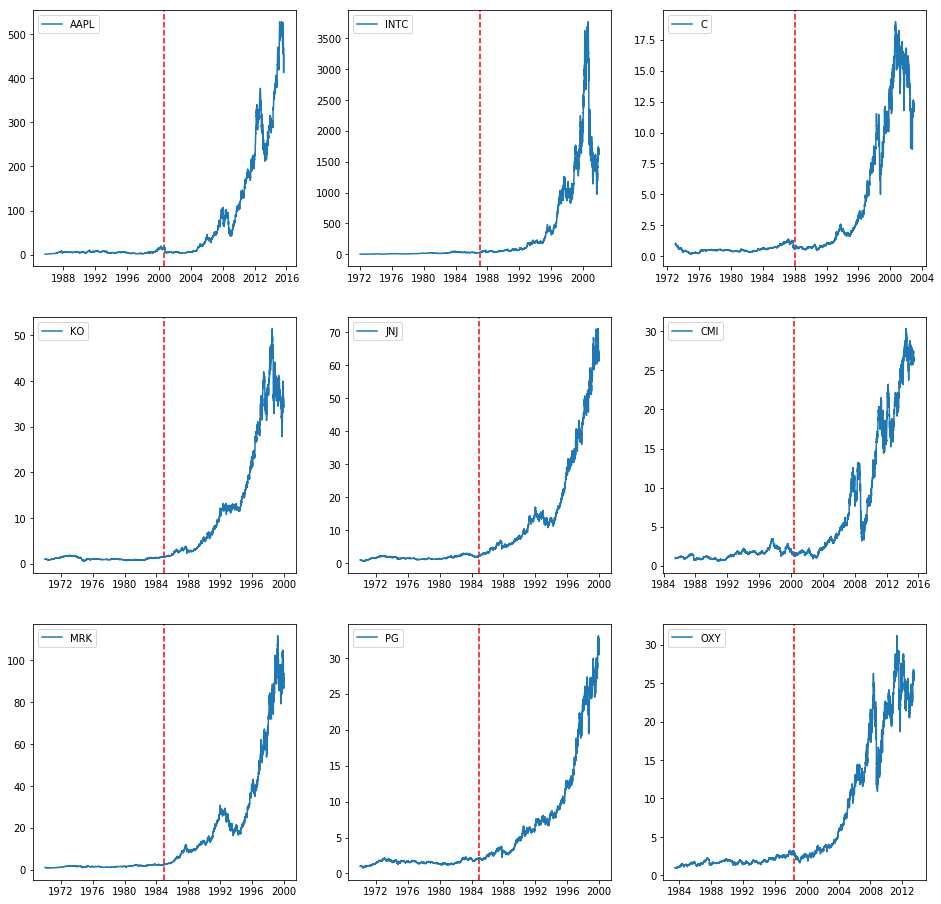
These plots are scaled such that $y_0 = 1$, i.e., the value of the stock at $y_t$ corresponds to the value at time $t$ of $1 invested at the start of the time span. So, for example, a dollar invested in Apple in 1986 would be worth about $450 in 2016. The dashed line is the 15-year “transition point” marker.
The tickers correspond to the following businesses:
- AAPL: Apple
- INTC: Intel
- C: Citigroup
- KO: Coca-Cola
- JNJ: Johnson & Johnson
- CMI: Cummins
- MRK: Merck & Co
- PG: Proctor & Gamble
- OXY: Occidental Petroleum
By this metric, none of the Good to Great companies show up. Interestingly, competitors of several of the Good to Great companies do: Citigroup (competes with Wells Fargo), Proctor & Gamble (competes with Kimberly-Clark), Merk & Co (competes with Abbott Laboratories), and Johnson & Johnson (competes with Kimberly-Clark, Abbott).
Unlike Jim Collins, we also have the benefit of hindsight at our time of writing. Let’s see how each of these business did after the 30-year time span we looked at:
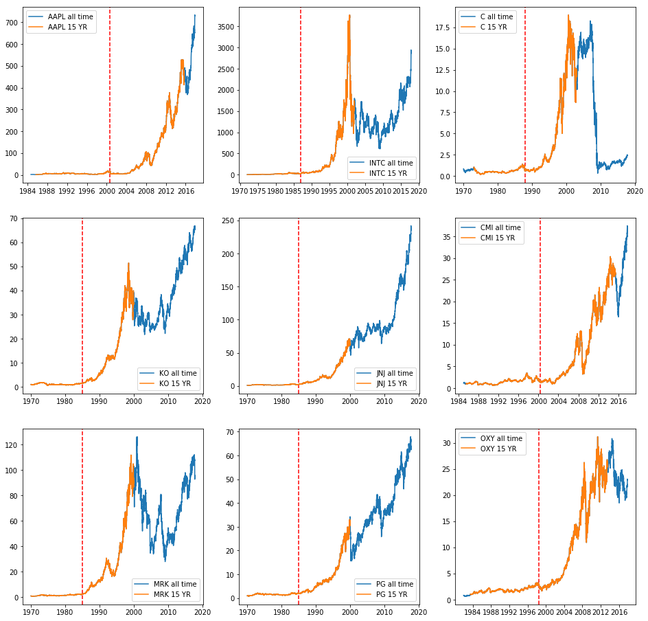
This last batch of plots cover different time spans, so the returns are not directly comparable. All the same, we see that this pattern of exponential growth is generally not sustainable; only about half of these companies’ stocks trade higher today than their peak over the time period observed, and most have experienced significant slowdowns outside of the 30-year window.
I’ll close this post by waxing philosophical for a few stanzas:
First, looking at historical stock movements to infer conclusions about causality (and in particular about what practices or actions are responsible for stock movements) is an inherently risky business—if you’re not extraordinarily careful, you’ll commit a post hoc fallacy or fall victim to the halo effect. Correlation does not imply causation, nor does it imply independence of the covariates.
Second, there’s an incredible amount of noise in stock movements and no company exists in a vacuum: it can be extremely difficult to distinguish the effects of intrinsic characteristics of a business from the market environment (and global ecosystem) that business exists in. Moreover, market dynamics evolve rapidly, so strategies that were effective at one point in time may not be in the future. Collectively, this means we should take a healthy grain of salt with any work that promises a common set of strategies for business success and bases its analysis primarily on internal factors.
Finally, management is not a physical or “hard” science, and we should be suspicious of any “grand unified theories of management” promising a reductive approach to business success (particularly when these theories come clothed in the trappings of science but without the accompanying rigor). At best, management theory is a social science, complete with all of the challenges that come with observational rather than experimental inference. Much like the social sciences, we should expect progress in our understanding to be messy, hard-won, and constantly evolving.
Good to Great was an interesting read with lots of good advice, but it’s best understood as a collection of case studies, not as the results of a rigorous scientific inquiry.