The Hurst Exponent
Consider a time series. How can you tell if the series is a random walk or not? One popular test is to compute the Hurst exponent. However, the Hurst exponent does not definitively characterize the “random-walkiness” of the series. In this post, I’ll define the Hurst exponent and explore what kinds of non-randomness it allows you to detect.
Two running examples
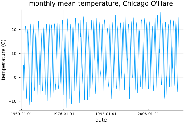
Let’s first introduce two examples of the kinds of time series we want to examine. We will return to these examples throughout this post. First, a climate dataset: the monthly average temperature measured at Chicago O’Hare airport, 1960–2020 (source).
And for our second time series example, the adjusted daily closing price of SPY, an exchange-traded fund closely tracking the S&P 500 index:
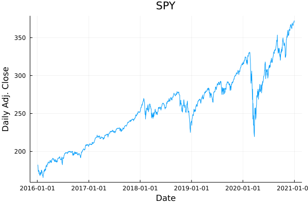
Qualitatively, it is very easy to distinguish these series from one another. In particular the Chicago temperature dataset exhibits clear seasonality, while SPY has apparently a strong positive bias. Is there a statistic that distinguishes between these two series? It turns out that there is, and, as you might guess from the title of this post, one such statistic is the Hurst exponent. But first, we need to think about how to model these time series.
Random walks
A random walk is a succession of random steps. An (arithmetic, real-valued) random walk can be described as follows:
- Let $\mathcal{D}$ be some probability distribution (e.g. a normal distribution).
- Let $y_0$ denote the initial value of the series.
- Then, \(y_{t} - y_{t-1} \sim \mathcal{D}\) describes an arithmetic random walk.
Equivalently, such a random walk can be written as
\[y_{t} = y_{t-1} + \varepsilon_{t}\]where $\varepsilon \sim \mathcal{D}$ is the “step”. (This is an arithmetic random walk because the steps are additive; geometric random walks can be constructed where the steps are multiplicative, and it is often possible to “translate” between the two frameworks by taking a logarithm or exponent.)
This kind of random walk has a few important properties. First, observe that the expected value at time $t$ is just $t$ times the mean value of the step distribution:
\[\mathbb{E}\left[ y_{t} \right] = y_0 + t \mathbb{E}\left[ \mathcal{D} \right]\]The second, related property is that $y_{t}$ depends only on $\mathcal{D}$ and $y_{t-1}$; in particular $y_{t-n}$ provides no predictive value whatsoever. So, these random walks satisfy a kind of Markov condition:
\[P(y_t | y_{0}, y_{1}, \ldots , y_{t-1}) = P(y_t | y_{t-1})\]From a time series modeling perspective, this property makes random walks both extremely simple and, as a practical matter, frustrating: the modeler cannot provide a better prediction for future values of the series than the equation above, regardless of the previous history of the series.
Detecting whether a particular series is a random walk is thus of extreme interest to anyone doing time series modeling! (And potentially profitable—for example, if you knew that SPY was not a random walk, you could construct a lucrative trading strategy!)
The Hurst exponent
Consider for a moment a generic time series \((y_0, y_1, \ldots, y_t, \ldots)\) . Let’s denote by \(\Delta_{t}\) the differences \(\Delta_{t} := y_{t} - y_{t-1}\). Then,
\[y_{t} = y_0 + \Delta_1 + \Delta_2 + \cdots + \Delta_t\]Suppose that each \(\Delta_t\) is a random variable. Then, as we saw above for a random walk,
\[\mathbb{E} [y_t] = y_0 + \sum_{i=1}^{t} \mathbb{E}[ \Delta_t ]\]However, this is not true for the variance. Recall that variance of a sum is
\[Var(X + Y) = Var(X) + Var(Y) + 2 Cov(X, Y)\]so our sum becomes
\[Var(y_t) = \sum_{i=1}^{t} Var(\Delta_t) + \sum_{i \neq j} Cov(\Delta_i, \Delta_j)\]If $y$ is a pure random walk with each \(\Delta_i \sim \mathcal{D}\) then
\[Var(y_t) = t Var(\mathcal{D});\]on the other hand, if \(Cov(\Delta_{t}, \Delta_{t+1}) > 0\), then
\[Var(y_t) > t Var(\mathcal{D}),\]and if \(Cov(\Delta{t}, \Delta_{t-1}) < 0\), then
\[Var(y_t) < t Var(\mathcal{D}).\]Therefore, if we have some observed time series, we can get a crude measure of the dominant type of autocorrelation by plotting $t$ against \(Var(y_t - y_0)\) for various choices of $t$. We should expect that
\[Var(y_{t + \tau} - y_{t}) \sim \tau^{2H}\]for some $H$. This $H$ is the Hurst exponent, where $H = 0.5$ is what we would expect to find if the series was a pure random walk (no significant positive or negative autocorrelation).
Rescaled range analysis
In practice, the Hurst exponent is often computed using the rescaled range. The rescaled range is essentially the “number of steps between the minimum and maximum of an interval.” For example, suppose that we had the following time series (generated from a pure random walk with \(\mathcal{D} = \mathcal{N}(0,1)\)):
  1.4866073437653307,
  0.26288465354836776,
 -1.3740853365602632,
 -1.693951275825174,
 -0.9242067975352728,
  0.1995408510873251,
 -0.48978979266680867,
 -0.8906229497127485,
 -0.2672740250657575,
 -0.4059957360532904
Then, the “deltas” (\(y_{t} - y_{t-1}\)) of our series are
 -1.223722690216963,
 -1.636969990108631,
 -0.3198659392649108,
  0.7697444782899012,
  1.123747648622598,
 -0.6893306437541338,
 -0.4008331570459398,
  0.623348924646991,
 -0.13872171098753294
The mean delta is -0.21, and the standard deviation is 0.92.
If we subtract off the mean delta, and divide by the standard deviation, we get the series
 -1.1008060608989385,
 -1.5496812468072312,
 -0.1190238030973122,
  1.0645267703141652,
  1.4490501269988194,
 -0.5203417015025235,
 -0.2069715645066769,
  0.90550980547293,
  0.07773767402676754
Taking the cumulative sum of this series, we get
-1.1008060608989385
 -2.65048730770617
 -2.7695111108034816
 -1.7049843404893166
 -0.25593421349049716
 -0.7762759149930206
 -0.9832474794996975
 -0.07773767402676746
  0.0
Then, the difference between the maximum value (0.0) of the summed series and the minimum value (-2.7695) gives us the rescaled range: 2.7695. Let’s call this quantity \(RR(y)\). Just like the variance, we should generally expect that
\[\mathbb{E}[RR(\tau)] \sim \tau^{H}\](where I am using \(RR(\tau)\) as shorthand for the rescaled range of a series of length $\tau$.)
Why use the rescaled range instead of estimating \(Var(y_{t + \tau} - y_t)\)?
One reason is that, empirically, the rescaled range provides a more stable estimate.
You can test this yourself at home: generate a pure random walk (e.g. by cumsum(randn(5000)) in Julia) and compute the Hurst exponent both ways.
In my testing, the exponent generated by the variance method tends to be quite a bit noisier than the rescaled range method.
Calculating the Hurst Exponent
Now let’s return to our example series: SPY and the Chicago O’Hare mean monthly temperatures. How closely do these series resemble a pure random walk? Do they exhibit momentum or mean-reversion?
SPY
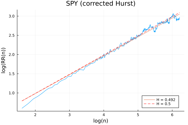
First, let’s look at SPY. To compute the Hurst exponent, we need to calculate the average rescaled range over various lengths $n$, and plot this against $n$. The slope of the log-log plot gives us the Hurst exponent:
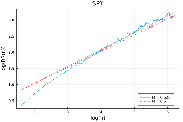
Above, the blue line is the observed data, the orange line the best-fit linear regression, and the dashed red line the slope of the line we would expect from a pure random walk. Here we find the best-fit slope to be \(H = 0.520\), which is very close to what we would expect from a pure random walk (\(H = 0.5\)).
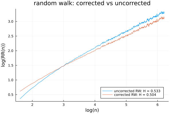
Looking more closely at the plot, it is notable that the slope is somewhat steeper in the low-$n$ region. You might initially guess that this suggests SPY exhibits some momentum over short time periods—but in fact, this is a statistical artifact that appears even for pure random walks:
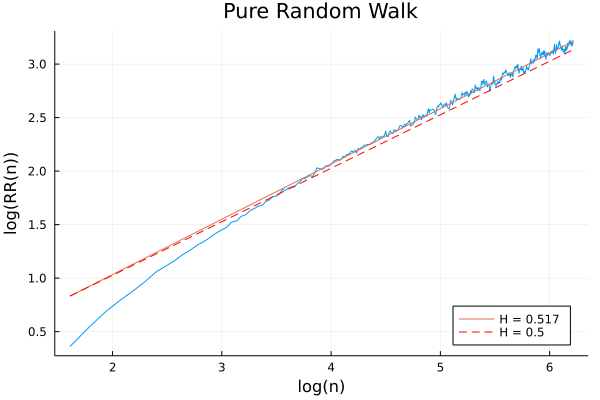
For this reason, Annis and Lloyd propose an adjusted rescaled range:
\[\mathbb{E}[RR(n)]=\begin{cases} \left(\frac{n-\frac{1}{2}}{n}\right)\frac{\Gamma(\frac{n-1}{2})}{\sqrt{\pi}\Gamma(\frac{n}{2})}\sum_{i=1}^{n-1}\sqrt{\frac{n-i}{i}}, & n\leq340\\ \left(\frac{n-\frac{1}{2}}{n}\right)\frac{1}{\sqrt{n\frac{\pi}{2}}}\sum_{i=1}^{n-1}\sqrt{\frac{n-i}{i}}, & n>340. \end{cases}\]To apply this adjustment to our calculation, subtract off the log Anis-Lloyd expected R/S from the empirically observed log rescaled range.
This has the effect of eliminating the “apparent momentum” at the left-hand side of our Hurst plots, as seen below for a pure random walk:
Applying this correction to SPY, the apparent momentum disappears, and we find a Hurst exponent of 0.492:
Chicago temperatures
Next let’s look at the Chicago temperature data, which was observably highly periodic.
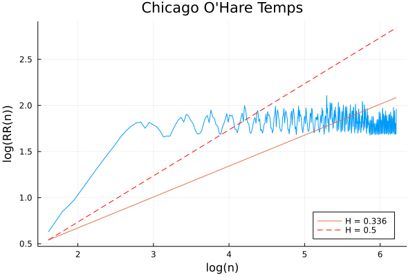
This Hurst exponent plot looks very, very different from the SPY and random walk ones! As $n$ increases above about $n = 20$, there is very, very strong mean reversion. This is as we expect: $n > 24$ consists of subsets with more than two year’s worth of temperature data, and, as evident from the original plot, the mean monthly temperature achieves its maximum difference over about 6 months (January to July); as $n$ increases, the rescaled range remains effectively constant.
So far so good—the Hurst exponent very clearly distinguishes between these two types of series. But, the Hurst exponent is not a panacea. Let’s look at another example.
The limitations of the Hurst exponent
Consider the following time series:
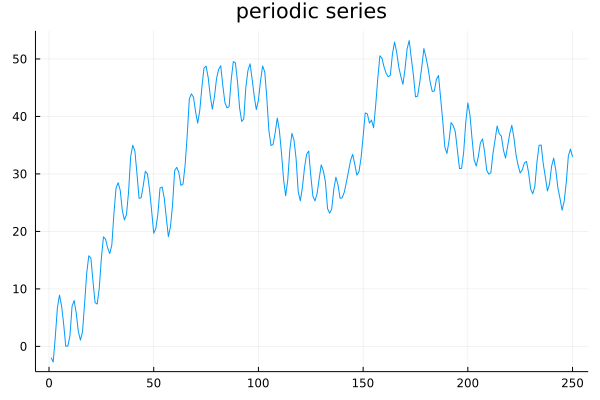
This series exhibits consistent short-term periodicity, but it is not stationary. The short-term periodicity is clearly evident in its autocorrelation plot:
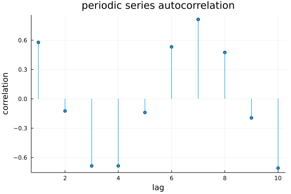
This is an autocorrelation plot of the differenced series (that is, the $\Delta_t$ from the beginning of the post). Notice how the autocorrelation plot resembles a sine wave: the next change in value for the series is positively correlated with the previous change, but negatively correlated with the delta from several steps ago, and then positively correlated with the delta from several steps before that, and so on.
From what we saw above with SPY (largely indistinguishable from a random walk) and Chicago mean monthly temperatures (strongly mean-reverting), we should expect this periodicity to be picked up by the Hurst exponent, right?
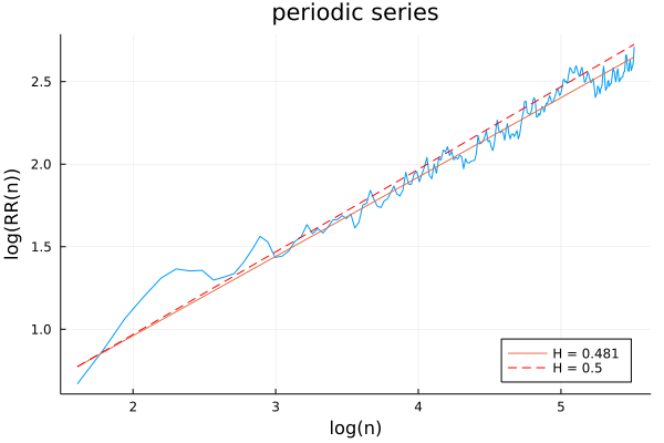
Wrong! The resulting Hurst exponent (either with or without the Annis-Lloyd correction; the above plot includes the correction) is very close to 0.5, and the plot is not very distinguishable from a random walk.
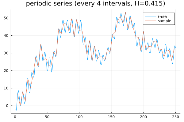
This is because the Hurst exponent is not only a function of the time series, it is also a function of the sampling frequency. If we sample the value of the series every 4 observations, then we get a lower Hurst (0.415), suggestive of mean reversion:
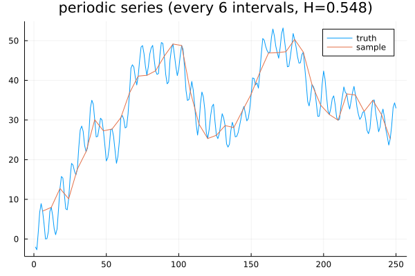
If, on the other hand, we sample every 6 observations, then we get a higher Hurst (0.548), suggestive of momentum:
The moral of the story is that, while the Hurst exponent can be a powerful tool, it does not definitively characterize the behavior of a given time series, nor can it be relied upon to distinguish a series from a random walk. More precisely, an \(H \neq 0.5\) suggests that the series is not a random walk; however, an \(H \approx 0.5\) does not imply the series is a random walk. And that’s the Hurst exponent!