Stochastic Gradient-free Descent in Julia
If you haven’t heard, Julia—the “Ju” in Jupyter—is a high performance numerical computing language. I have heard it said that Julia is great (and I believe everything I read on Hacker News). Julia also has a pretty slick deep learning library called Flux, which comes built in with the automatic differentiation magic and CUDA support we all love in our Python deep learning packages. So, let’s give it a whirl and see if Julia is all it’s cracked up to be. As is apparently becoming a theme for me, I’ll do this in the dumbest way possible.
BUT WAIT! I thought Python was the most bestest language for data science, why should I care about Julia?
Maybe a better question is, why do you use Python for data science?
It’s largely a historical accident that Python has become so dominant in data science (and machine learning, specifically). Some of the earliest instances of what is now called data science emerged in the physics community in the 80s and 90s. High-energy physics (like the kind involved in the detection of the top quark) in particular often involves munging through huge datasets, such as those generated by particle detectors. Physicists needed to combine efficient, performant numerical computation packages to do their research, and most of the libraries implementing these types of computations were written in languages like C and Fortran. C and Fortran have many virtues, but ease of use is generally not counted among them.
Enter Python. Python, a dynamically typed language with simple foreign function interfaces, provides an excellent connective tissue to stitch together heterogeneous collections of numerical libraries into a single package. Eventually, libraries like NumPy emerged. These libraries were purpose-built for that kind of stitching, where high-level code is written in easy Python, and the underlying numerical crunching takes place in some distant C function away from a data scientist’s prying eyes.
And this is largely how Python is still used—if you’ve looked at the source code behind packages like TensorFlow, PyTorch, or spaCy, you’ll notice that most of the code isn’t in Python, and the bits that are “Python” often use optimizations like Cython for performance.
Which brings us to the promise of Julia. What if, instead of gluing together code from a bunch of languages using a slow, dynamically typed, interpreted scripting language, we did our data science in a language designed to for that purpose?
To explore that possibility, I ran a short experiment to replicate a typical deep learning workflow in Julia.
An example
To start with, I’m going to build a classifier to guess whether or not a particular passenger survived the Titanic. There will be two parts to this example:
- I’ll build a feedforward classifier and train it via gradient descent; and
- I’ll build a feedforward classifier and train it via stochastic gradient-free descent.
By stochastic gradient-free descent, I mean the following: at each update step, I will update the model parameters using a randomly chosen vector (rather than the gradient of the loss function). If this random step improves the loss, I will use those parameters. If this random step does not improve the loss, I will fall back to the previous parameters. This algorithm has three desirable properties:
- It is highly inefficient, and thus will exercise Julia’s vaunted performance;
- It is not straightforward to implement in PyTorch or TensorFlow; and
- It’s mildly hilarious in the same way a bubble sort is.
Let’s begin.
Data munging
Start by loading in some libraries that we need. Julia does some precompilation when loading, so if you’re following along in a notebook, you’ll notice that this is frustratingly slow.
using Statistics; # for... statistics
using Random;     # for sampling
using CSV;        # to load in CSV files
using DataFrames; # does what it says on the tin
using Flux;       # for "deep" learning
using Plots;      # so we have something to show for our efforts
(Python users: it’s helpful to put a semicolon ; at the end of most lines, otherwise the last line in your REPL will be printed to the notebook or terminal—this can be obnoxious if you’re manipulating a large dataframe.)
Now we can load in our dataset:
df = CSV.read("titanic.csv");
describe(df)
| variable | mean | min | median | max | nunique | nmissing | eltype |
|---|---|---|---|---|---|---|---|
| :PassengerId | 446.0 | 1 | 446.0 | 891 | nothing | nothing | Int64 |
| :Survived | 0.383838 | 0 | 0.0 | 1 | nothing | nothing | Int64 |
| :Pclass | 2.30864 | 1 | 3.0 | 3 | nothing | nothing | Int64 |
| :Name | nothing | “Abbing, Mr. Anthony” | nothing | “van Melkebeke, Mr. Philemon” | 891 | nothing | String |
| :Sex | nothing | “female” | nothing | “male” | 2 | nothing | String |
| :Age | 29.6991 | 0.42 | 28.0 | 80.0 | nothing | 177 | Union{Missing, Float64} |
| :SibSp | 0.523008 | 0 | 0.0 | 8 | nothing | nothing | Int64 |
| :Parch | 0.381594 | 0 | 0.0 | 6 | nothing | nothing | Int64 |
| :Ticket | nothing | “110152” | nothing | “WE/P 5735” | 681 | nothing | String |
| :Fare | 32.2042 | 0.0 | 14.4542 | 512.329 | nothing | nothing | Float64 |
| :Cabin | nothing | “A10” | nothing | “T” | 147 | 687 | Union{Missing, String} |
| :Embarked | nothing | “C” | nothing | “S” | 3 | 2 | Union{Missing, String} |
Anyone who has spent a couple of minutes on Kaggle will be familiar with this dataset, and anyway, for this exercise, we don’t care about building the perfect predictor of Titanic deaths.
First though, a baseline: about 38.4% of passengers survived on the Titanic. That means that a baseline classifier that assumes everyone on the Titanic died will be correct about 61.6% of the time. So, if our accuracy is less than 61%, we’ve done something very wrong.
Next, let’s subset to just numeric features (we’ll add in categoricals in a second):
X = df[["Age", "Fare", "SibSp"]];
Add in the Sex field:
X["Sex"] = (df["Sex"] .== "male")
Note the use of the dot in “.==”.
This is a very cool feature of Julia!
The dot operator is more properly called the broadcast operator.
This allows you to apply functions to arrays elementwise.
Here, I’ve only used an equality check, but these functions can be arbitrary and user-defined.
This is analogous to the .apply() method in Pandas, except that unlike Pandas, it’s actually vectorized and fast.
Next, let’s one-hot encode the Embarked feature:
for col in ["Embarked"]
    vals = unique(df[col])
    for val in vals
        if !ismissing(val)
            X[col * "_" * string(val)] = (df[col] .== val)
        end
    end
end
I’ve structured this as a loop over a list of categorical features, so you could apply it to other features as well (e.g. Name, if you’re some kind of maniac).
Train/test split
Now, let’s split the data into training and testing subsets. I’ll do this by picking a random index for each set:
idx = randperm(nrow(df))
train_idx = idx[1:round(Int, 0.8*nrow(df))]
test_idx = idx[round(Int, 0.8*nrow(df)):nrow(df)]
A couple of comments about this:
nrowis a function that counts the number of rows in a dataframe (not sure whylengthdoesn’t do this), andrandpermconstructs a random permutation of all of the integers between 1 andnrow(df).- Array indices in Julia are one-based instead of zero-based, i.e. you access the first element of an array with
arr[1], notarr[0]. This is the same convention as R and Matlab, but obviously not the same as in C-like languages (such as Python). - Unlike slices in Python, slices in Julia include the last element (see above about 1-based indexing), and the last index has to be specified.
arr[123:]is unfortunately not valid, and neither isarr[:-3].
Before we can build a model, we should also deal with missing data, and rescale & center our numeric fields. Let’s define a function to do these things:
function rescalefield(X, fieldname)
    X[fieldname] = coalesce.(
        X[fieldname], mean(
            skipmissing(X[train_idx,:][fieldname])
            )
        )
    x_mean = mean(X[train_idx,:][fieldname])
    x_std = std(X[train_idx,:][fieldname])
    X[fieldname] = (X[fieldname] .- x_mean) ./ x_std
end
The first line of this function handles missing elements.
The skipmissing function produces an iterator that ignores the missing values in the specified column.
This way, mean won’t have NaNs or missings floating around in it.
Then, coalesce converts missing or invalid values into the specified value (in this case, the mean of the field).
(Note the use of the broadcast operator to apply this elementwise!)
The second line of this function centers and rescales this column to have mean 0 and standard deviation 1.
Apply this to our numeric fields:
rescalefield(X, "Age");
rescalefield(X, "Fare");
rescalefield(X, "Sibsp");
Pro tip: The training index shows up in this function for a reason! Specifically, the mean and standard deviation are drawn from the training sample, not the test sample. This way, no information about the test sample accidentally gets leaked to the model during training. (Imagine you’re doing inference live, one record at a time: how would you know what values to transform by?)
Finally, let’s clean up any leftover missing values that somehow slipped through our nets by setting them to 0.
X = coalesce.(X, 0)
Deep learning in Flux
Flux provides an interface for model construction that will feel very reminiscent to any user of PyTorch or Keras. I’m defining a simple dense feedforward network with ReLu activations for the hidden layers and a sigmoid activation for the output.
model = Chain(
    Dense(7, 256, relu),
    Dense(256, 256, relu),
    Dense(256, 1, sigmoid)
    )
Next, let’s set up the optimizer.
optim = Flux.Optimise.ADAM()
wts = Flux.params(model)
The Flux.params() function defines a collection of parameters.
Since we’ve constructed this model using Flux’s built-in Chain function, this automatically selects the parameters we’re interested in.
But, if you wanted to, you could also explicitly construct the collection of parameters from the tensors involved.
This is a binary classification problem, so the loss function I’ll use is binary cross entropy:
criterion(u, v) = Flux.Losses.binarycrossentropy(model(u), v)
(It’s a little more efficient to have the model produce logits and use logitbinarycrossentropy instead, but this example isn’t really intended for production use.)
Let’s also prepare our input data and targets:
X_in = transpose(convert(Matrix{Float32}, X))
y = transpose(convert(Array{Float32}, df["Survived"]))
Note that I’m transposing the arrays in both cases! This is because, in contrast to arrays in NumPy or PyTorch, multidimensional arrays in Julia are stored on column-major order. One way to remember this is that in Julia, a 1-dimensional vector is a column, whereas in NumPy, it’s a row. Hence, our input records should correspond to columns in the input matrix, not rows.
Since reading binary cross entropy scores isn’t as intuitive as classification accuracy (at least for me), let’s also define an accuracy function to measure our performance:
accuracy(x, y) = sum(round.(model(x)) .== y)/length(y)
With that out of the way, we’re ready to start training. Here’s the training loop, with early stopping:
last_loss = crit(X_in[:, test_idx], y[:, test_idx])

for epoch = 1:1000
    # compute the gradient of the loss criterion
    grads = gradient(wts) do
        criterion(X_in[:, train_idx], y[:, train_idx])
    end

    # update the model parameters
    Flux.update!(optim, wts, grads)

    # stop early if we are seeing degrading test performance
    # (and we've trained for at least 100 epochs)
    new_loss = criterion(X_in[:, test_idx], y[:, test_idx])
    if (new_loss > last_loss) && (epoch > 100)
        break
    end
    last_loss = new_loss
end
For me, this stops after 105 iterations due to degrading test performance. Here are the training curves:
plot(1:length(train_losses), train_losses, label="Train")
plot!(1:length(test_losses), test_losses, label="Test")
xlabel!("Iteration")
ylabel!("Loss")
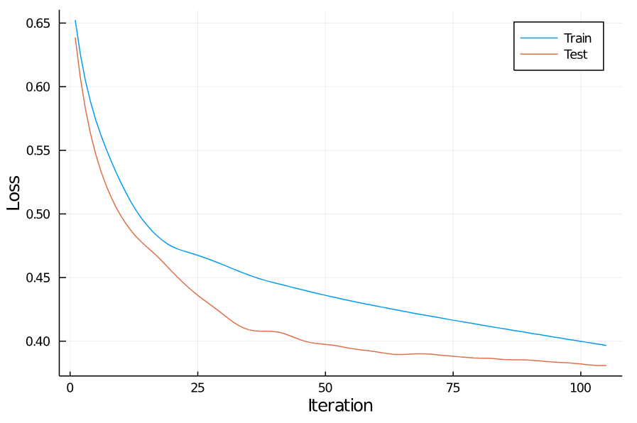
Training concludes with a training loss of 0.401, corresponding to an accuracy of 82.3%.
Performance on the test set is actually slightly better: the loss is 0.382, corresponding to an accuracy of 86.0%.
Probably not good enough to win any Kaggle competitions, but not bad!
Gradient-free descent
Now, on to the silly part of this blog. Here’s the update step of the training loop, where we modify the parameters by the gradient vector:
grads = gradient(wts) do
    criterion(X_in[:, train_idx], y[:, train_idx])
end

Flux.update!(optim, wts, grads)
We’re going to modify the training loop to discard the gradient and Adam optimization entirely, and instead advance in a random direction.
First, here’s a function to produce a random vector to apply to our parameters:
function randstep(parameters, std)
    parameters = deepcopy(parameters)
    for par in parameters
        par .= par .+ (std .* randn(size(par)))
    end
    return parameters
end
Next, let’s write the training loop. The basic idea is the following: Let $\theta_{t}$ denote the model parameters at each iteration, and $\pi(\theta_{t})$ the model function given those parameters. Then, for each step of the iteration:
- Pick $n$ random vectors $\delta_{k}$, $k = 1, \ldots, n$.
- Construct $n$ model candidates $\pi_{k} (\theta_{t})$, where \(\pi_{k} (\theta_{t}) := \pi (\theta_{t} + \delta_{k})\)
- Update $\theta_{t}$ by \(\theta_{t+1} := \arg \max_{k} \mathcal{L}(\pi_{k}(\theta_{t}))\)
This is a very simple example of a genetic algorithm, where each iteration corresponds to a generation of the population, and each individual has a single parent. If we know that the loss hypersurface is convex, then it’s also a much less efficient way of traversing the parameter space!
In fact, our implementation will differ slightly from the one above: we’ll check each descendent one at a time, and if any descendent is better than the parent, we’ll immediately update to that child. For large $n$, this is significantly more efficient early in training than checking every possible descendent because, assuming you started from a random point, any random direction has about a 50% chance of improving your loss.
Here’s the code:
baseline = deepcopy(Flux.params(model))
baseline_loss = criterion(X_in[:, train_idx], y[:, train_idx])

for epoch = 1:500

    for k = 1:100
        new_wts = randstep(baseline, 0.01)
        Flux.loadparams!(model, new_wts)
        new_loss = criterion(X_in[:, train_idx], y[:, train_idx])

        if(new_loss < baseline_loss)
            baseline = deepcopy(new_wts)
            baseline_loss = new_loss
            break
        end

        # if, somehow, none of these directions improve things, then halt
        # and try again on the next iteration
        if k == 100
            Flux.loadparams!(model, baseline)
        end
    end
end
And here are the training curves:
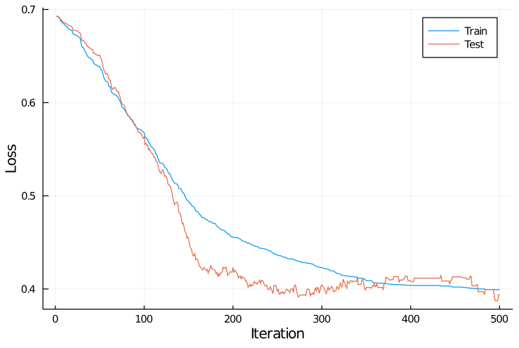
Notice the long plateaus near iteration 400 where the training and test loss were constant—these are areas where none of the 100 random directions selected improved performance.
(These are especially visible in the orange test curve.)
This approach was significantly slower than gradient descent: it took about 500 iterations before performance began to plateau, and each iteration involved evaluating the loss criterion a hundred times (as opposed to once in gradient descent).
Still, Julia is fast!
The entire calculation took less than a minute on my local machine.
Compared to optimization techniques based on gradient descent, this approach also has a number of parameters to tune that are highly sensitive to the complexity of the model, such as the step size and number of samples per iteration (here, 0.01 and 100, respectively).
The repeated use of deepcopy() and loadparams! suggests that this kind of thing is not what Flux is really designed for, either.
Nevertheless, the final performance ended up pretty respectable: 82.7% accuracy on the training set, and 86.6% accuracy on the test set.
And we didn’t have to calculate a single gradient!
(At least not explicitly…)
Is there any reason you’d ever want to do this for real?
Probably not?
The big issue with gradient descent is that convergence to a global optimum is only guaranteed when the loss surface is convex, and this is often not the case with neural nets. In theory, by taking gradient-free random steps, you can “walk out of” a local minimum, rather than get trapped like you would with gradient descent. But therein lies the rub: to determine which descendent’s parameters we use for the update, we use the criterion to evaluate the descendent. Thus, the only way our descendent can walk out of the well is if the step size is sufficiently large as to get back on “flat ground.”
Moreover, conventional thinking suggests that, for neural nets, in most cases true local minima (where all gradients vanish, and the Hessian is positive semidefinite) are few and far between, so you shouldn’t really worry about getting stuck.
In closing, what have we learned? First, let’s brag that we can predict who survived on the Titanic with up to 86% accuracy using deep learning! This is, of course, only 14% worse than actual historians are able to manage. Second, it’s hopefully clear that Julia is a slick language, and I’d argue that it broadly feels like a better fit for data science work than Python. (Definitely true when you restrict yourself to the standard library, and still feels mostly true even when you allow third party packages.)
Python has a huge community, historical legacy, and the weight of some massive corporate-sponsored projects behind it, so it’s unlikely that Julia will ever overtake it. (Maybe, if we’re lucky, it will finally kill R…) But, hopefully, it will find a place in the sophisticated, discerning data scientist’s repertoire.