Simulating COVID-19 (like an idiot)

Written on March 22, 2020

Like many Americans, I’ve been locked up at home the past few weeks watching the coronavirus public health crisis unfold. (Luckily, for now nobody I know has yet been affected.) One of the things I’ve found hardest about this crisis is just the uncertainty surrounding all of the data: how dangerous is COVID-19? How many people will catch the virus? How likely am I to catch it? How long will my family be stuck at home?

With some time on my hands, I decided to put together some very naive simulations of possible scenarios, under various simplifying assumptions. Before reading further, let me emphasize: I am not an epidemiologist!!! For a (sobering) and more rigorous analysis, check out the non-pharmaceutical intervention modeling done at Imperial College London. The analysis of this post is purely speculative and makes a number of (likely incorrect) simplifying assumptions, and one of the key takeaways of this exercise is just how sensitive these scenarios are to each of the parameters.

If you’re not interested in the technical details of the simulation, you can skip straight to the results—although again, I offer the disclaimer that none of this is particularly accurate or predictive!

Key parameters

A review study published in JAMA provides the following estimates for key parameters of the virus:

The incubation period for the virus is estimated to be between 1 and 14 days (although possibly up to 24 days), with a median of 5 to 6 days. The incubation period is the length of time between when a patient is infected with the virus and when symptoms begin.
The reproductive number ($R_0$) is estimated to be between 2 and 3. The reproductive number is the expected number of secondary cases produced by a single infected person in a susceptible population. [source]
The case fatality rate (CFR) is estimated to be between 1 and 2% [source], or between 1.8% and 3.4% in America [source] (note that this is heavily impacted by population demographics).
About 80% of cases are mild (not requiring hospitalization) and 20% are severe or critical.
The median time from onset to clinical recovery for moderate cases is 2 weeks and for severe or critical cases is 3 to 6 weeks. Among patients who have died, the time from symptom onset to outcome ranges from 2 to 8 weeks. [source]

Preliminary data from the CDC suggests that case outcomes are not significantly different in the US as compared to data reported by the earlier WHO investigation:

In particular, the CDC study provides the following table of outcomes:

Age group (years) (no. of cases)	Hospitalization	ICU admission	Case-fatality
0–19 (123)	1.6–2.5	0	0
20–44 (705)	14.3–20.8	2.0–4.2	0.1–0.2
45–54 (429)	21.2–28.3	5.4–10.4	0.5–0.8
55–64 (429)	20.5–30.1	4.7–11.2	1.4–2.6
65–74 (409)	28.6–43.5	8.1–18.8	2.7–4.9
75–84 (210)	30.5–58.7	10.5–31.0	4.3–10.5
≥85 (144)	31.3–70.3	6.3–29.0	10.4–27.3
Total (2,449)	20.7–31.4	4.9–11.5	1.8–3.4

The WHO found that about 80% of infected patients have mild to moderate disease (not requiring hospitalization), about 13.8% have severe disease requiring hospitalization, and 6.1% cases are critical. [source]

Simplifying assumptions

In order to start simulating an outbreak, let’s make some simplifying assumptions. Here they are:

During the incubation period, the probability of an infected person infecting another person is constant (i.e. an infected person is equally likely to spread the virus on day 1 of the incubation period as on day 8).
Once a sick person shows symptoms, they are quarantined and no longer infect any others.
Once a sick person shows symptoms, their probability of succumbing to the virus is constant (i.e. each day a sick person has a constant chance of dying, until they recover).
Once a sick person has recovered, they cannot be re-infected with the virus.
An infected person will infect only one other person per day during the incubation period.
The incubation period is given by a log-normal distribution with median at 6 days and 95% of the mass to the left of 21 days.
The recovery period for a case is given by a log-normal distribution with median at 18 days and 95% of the mass to the left of 42 days.

Obviously, these assumptions are not realistic!

Assumption 6 gives a log-normal distribution with parameters $\mu = \log(6) \approx 1.792$, $\sigma \approx 0.75$. Assumption 7 gives a log-normal distribution with parameters $\mu = \log(18) \approx 2.89$, $\sigma \approx 0.5$.

Using assumptions 1 and 5, we can figure out what the probability of an infected person infecting another person is:

\[R_{0}=\mathbb{E}\left[P(infect) \cdot N_{days}\right]\] \[=\int_{0}^{\infty} P \cdot x \left(\frac{1}{x\sigma\sqrt{2\pi}}\exp\left(-\frac{(\ln x-\mu)^{2}}{2\sigma^{2}}\right)\right)dx\] \[= P\exp\left(\mu+\frac{\sigma^{2}}{2}\right)\]

Hence

\[P=R_{0}\exp\left(-\mu-\frac{\sigma^{2}}{2}\right)\]

Using an $R_{0}$ of 2.4, this gives:

\[= 0.302\]

That is, an infected person has about a 30% chance of infecting one other person on any given day during the incubation period.

We can repeat the same grim calculation to determine the probability of dying during the recovery period, using the CFR:

\[CFR = \mathbb{E}\left[P(death)N_{days}\right]\] \[= P \exp\left(\mu + \frac{\sigma^{2}}{2}\right)\] \[P = 0.00098\]

That is, assuming a CFR of 2%, a constant chance of dying during the recovery period, and a log-normally distributed recovery time with a median of 18 days, the chance of dying on any given day during the recovery period is 0.098%.

Simulation Methodology

My simulation methodology is simple and crude: I begin with a population of size $N$. Each individual has a current state—one of healthy, incubating, sick, recovered, or dead. In addition, for each individual, I calculate the following properties:

An $R_0$, sampled uniform randomly from the interval [1.5, 3.3]
A CFR, sampled uniform randomly from the interval [1.8, 3.5]
An incubation period, sampled from the log-normal distribution with $\mu = \log (6)$ and $\sigma = 0.75$
A recovery period, sampled from the log-normal distribution with $\mu = \log (18)$ and $\sigma = 0.5$

Using the $R_0$ and $CFR$, for each person, I then calculate the daily probabilities of infecting another person and of dying if sick. Next, I initialize the simulation by infecting a single person.

Each day, I update the simulation: each sick person progresses through an incubation period to a symptomatic period, which terminates in either recovery or death. During the incubation period, each sick person may infect another, according to the probability calculated above. During the symptomatic period, each sick person may die, according to the probability calculated above.

In total, for each person, I track a 11 pieces of information:

The current state (5 boolean values)
The incubation period length
The recovery period length
The daily infection probability
The daily fatality probability
Days spent in incubation
Days spent symptomatic and recovering

Implementing the simulation

A naive (read: the dumb thing I tried first) approach to implementing this simulation would be to define a class to represent a member of the simulated population, and assign methods to that class to handle updates, infections, and change of state. For example, something like this:

class Pop(object):

    def __init__(self, inc_period, sick_period, p_infect, p_death):
        self.day = 0
        self.state = HEALTHY
        self.inc_period = inc_period
        self.sick_period = sick_period
        self.p_infect = p_infect
        self.p_death = p_death
        self.days_inc = 0
        self.days_sick = 0
    
    def step(self, population):
        if self.state == HEALTHY:
            return
        
        if self.state == INCUBATING:
            t = random.random()
            if self.p_infect > t:
                population.infect_someone()
            self.days_inc += 1
            if self.days_inc > self.inc_period:
                self.state = SICK
            return
        
        if self.state == SICK:
            t = random.random()
            if self.p_death > t:
                self.state = DEAD
                return
            self.days_sick += 1
            return

In practice, this approach is inefficient and does not scale well to large population sizes. Instead, we can use NumPy to write faster and more efficient code.

The basic idea is to keep track of the whole population in a single NumPy array, where each row is one person in the population, and each column corresponds to one of the 11 values we’re tracking. Let’s start by defining our parameters:

cfr_est = 0.0265
cfr_err = 0.0085

r0_est = 2.4
r0_err = 0.9

inc_mu = math.log(6)
inc_sigma = 0.75

rec_mu = math.log(18)
rec_sigma = 0.5

For convenience, I also hard-coded the indices of the various features each member of the population has:

STATE_HEALTHY = 0
STATE_INCUBATING = 1
STATE_SICK = 2
STATE_RECOVERED = 3
STATE_DEAD = 4

SICK_PERIOD = 5
REC_PERIOD = 6

PROB_INFECT = 7
PROB_DEATH = 8

DAYS_INC = 9
DAYS_SICK = 10

Now, let’s initialize the population:

def init_population(pop_size, 
                    cfr_est, 
                    cfr_err, 
                    r0_est, 
                    r0_err, 
                    inc_mu, 
                    inc_sigma, 
                    rec_mu, 
                    rec_sigma):
    population = np.zeros(shape=(pop_size, 11))
    population[:,STATE_HEALTHY] = 1
    population[:,INC_PERIOD] = np.random.lognormal(
        mean=inc_mu, sigma=inc_sigma, size=(pop_size,))
    population[:,SICK_PERIOD] = np.random.lognormal(
        mean=rec_mu, sigma=rec_sigma, size=(pop_size,))

    cfr = np.random.uniform(low=cfr_est - cfr_err, 
                            high=cfr_est + cfr_err, size=(pop_size,))
    r0 = np.random.uniform(low=r0_est - r0_err, 
                           high=r0_est + r0_err, size=(pop_size,))

    population[:,PROB_INFECT] = r0*math.exp(-inc_mu - (inc_sigma**2)/2)
    population[:,PROB_DEATH] = cfr*math.exp(-rec_mu - (rec_sigma**2)/2)
    return population

For a given set of general parameters (population size and our estimates and margins of errors for various features of the population), this function constructs a population matrix of healthy individuals and computes individual daily probabilities of infection and death, as well as duration of incubation and sick periods.

Next, a function to infect a given number of random healthy individuals in the population:

def infect(population, count):
    to_infect = np.random.choice(len(population), size=count, replace=False)
    infectees = to_infect[(population[to_infect,STATE_HEALTHY] == 1).nonzero()[0]]
    
    population[infectees, STATE_HEALTHY] = 0
    population[infectees, STATE_INCUBATING] = 1
    return

The one sneaky thing going on here is the .nonzero()[0] call:

population[to_infect,STATE_HEALTHY] == 1

returns a boolean array of the same shape as population, and we want to select the indices of the true values. .nonzero() returns the indicies of nonzero values, but it returns a tuple—and we’re only interested in the first element of that tuple.

Finally, let’s define the function to update the population array with each new day:

def step(population):
    infectious = (population[:,STATE_INCUBATING] == 1).nonzero()[0]
    sick = (population[:,STATE_SICK] == 1).nonzero()[0]
    population[infectious,DAYS_INC] += 1
    population[sick,DAYS_SICK] += 1
    
    # infect other people
    thresh_infect = np.random.uniform(size=infectious.shape)
    infects_others = len(
        (population[infectious,PROB_INFECT] > thresh_infect).nonzero()[0])
    infect(population, count=infects_others)
    
    # roll to live
    thresh_die = np.random.uniform(size=sick.shape)
    dies = sick[(population[sick, PROB_DEATH] > thresh_die).nonzero()[0]]
    population[dies, STATE_SICK] = 0
    population[dies, STATE_DEAD] = 1
    
    # move from infectious to sick
    new_sick = infectious[(
        population[infectious, DAYS_INC] > population[infectious,INC_PERIOD]
        ).nonzero()[0]]
    population[new_sick,STATE_INCUBATING] = 0
    population[new_sick,STATE_SICK] = 1
    
    # move from sick to recovered
    new_recovered = sick[(
        population[sick, DAYS_SICK] > population[sick, SICK_PERIOD]
        ).nonzero()[0]]
    population[new_recovered, STATE_SICK] = 0
    population[new_recovered, STATE_RECOVERED] = 1

Here again, I’m using the .nonzero() trick to get indices out. To transition between incubating and sick members of the population, and between sick and recovered members, I apply this trick twice. Also, at each step, for both incubating and sick population members, we roll a random number to determine whether or not the infection spreads, or someone dies, respectively.

To run a simulation, just walk through the step function for as long as you like. For example, for 120 days, an initial population of 1 million people, with 10 infected:

pop_size = 1_000_000
init_infected = 10

pops = init_population(pop_size, 
                       cfr_est, cfr_err, 
                       r0_est, r0_err, 
                       inc_mu, inc_sigma, 
                       rec_mu, rec_sigma)

infect(pops, init_infected)

for day in range(0, 120):
    step(pops)

The results

Running the simulation with the parameters gives me the following results:

Simulation 1

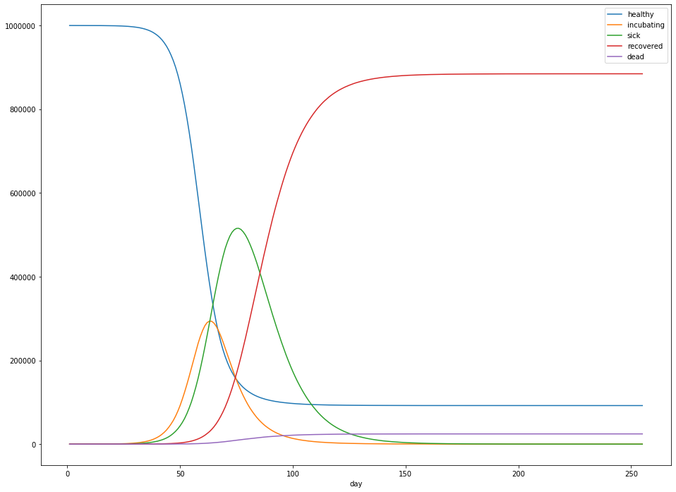
In particular:

Overall, 884,326 people were infected – 88.4% of the population.
The peak number of sick people was 515,541 – 52% of the population.
The peak occured 70 days after the first sick case was observed.
After 300 days, about 24,433 people had died – 2.4% of the population.
Sick cases generally lagged the number of incubating cases by about 5 days.
For cases that ended in death, death generally resulted after about 14 days of illness.
When the person survived, recovery generally occurred after about 21 days of illness.

These numbers were fairly stable across multiple runs of the simulation.

In Chicago, the first instance of community spread of COVID-19 occurred on March 8th. Social distancing measures such as school closures were enacted on March 17th, after 160 reported cases, and a statewide shelter-in-place directive was issued on March 21st, with 753 reported cases in the state and 14 days from the first instance of community spread.

Let’s explore the effect of similar policies. The simulation above can be seen as the “worst case” scenario, where we choose complete inaction. Let’s consider what happens in a good scenario, where social distancing measures are able to reduce the average $R_0$ from 2.4 to 1.2 (that is, incubating persons become half as likely to infect another person as they were previously). For the purposes of the simulation, I’ll assume that the measures are enacted 3 weeks into the simulation.

Simulation 2

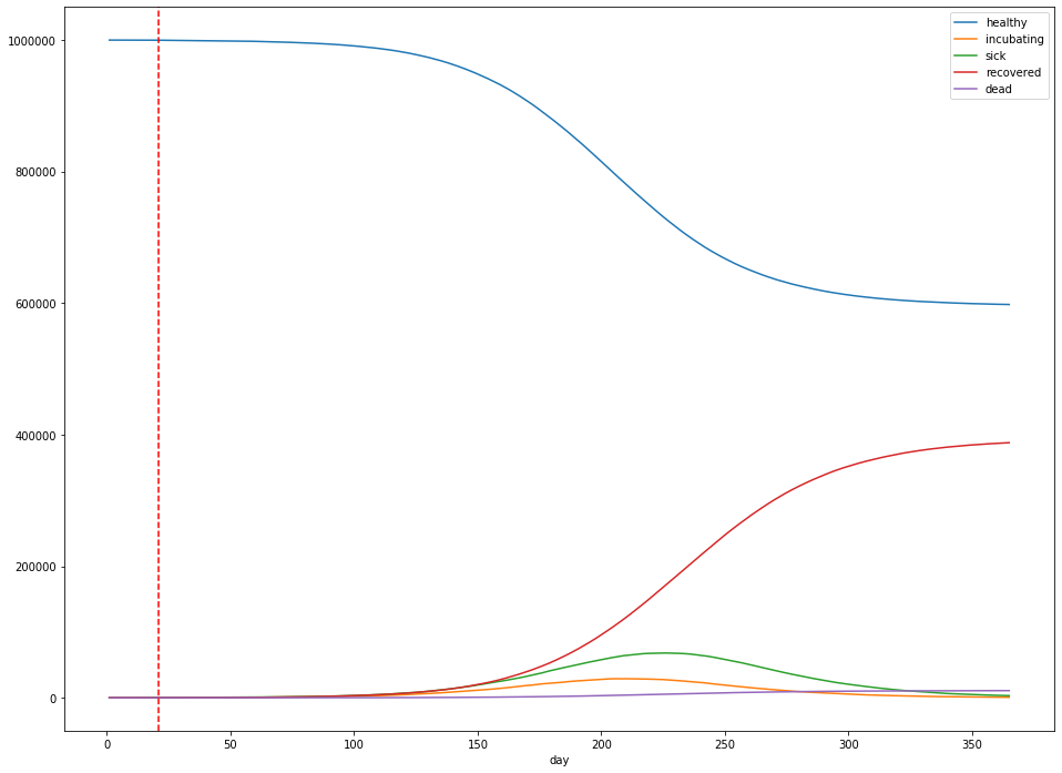
The total number of infections was 387,802 – 38.8% of the population.
The peak number of infected is 68,045 – 6.8% of the population.
The peak occurs 225 days after the first sick case is observed.
After 365 days, about 10,841 people had died – 1.08% of the population.

Under the assumptions of our simulation, varying the time the measures are enacted has a significant impact on the time at which the peak number of sick persons occurs: Moving the social distancing measures a week earlier (to 14 days into the simulation) pushes out the peak 3 weeks (to 220 days into the simulation). It doesn’t affect the height of the peak—instead, this is controlled by the effectiveness of the measures themselves.

For example, measures that reduce $R_0$ from 2.4 to 1.2 (above) result in a peak number of cases that’s 86% lower than without any measures at all, whereas reducing from 2.4 to 1.8 result in a peak number of cases of 336,169, only a 35% reduction in peak height (below).

Simulation 3

When can we stop?

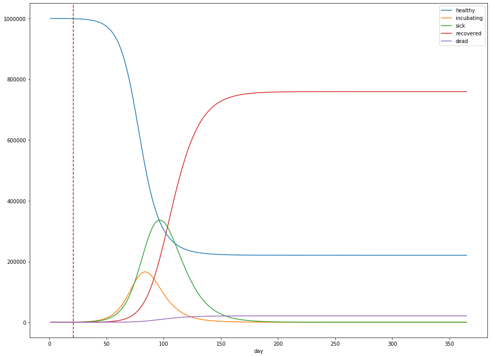
Imagine that we enact strict social distancing measures starting three weeks after the first reported sick case, and lasting for 60 days. After 60 days, we let up again. What happens?

Simulation 4

The dashed red lines in the figure above indicate the start and stop of social distancing measures, which are assumed to reduce $R_0$ to 1.2. Unfortunately for us, all this does is delay the peak: the peak number of sick patients is still close to 50% of the population (at 501,244), but at least the peak occurs 123 days into the simulation, rather than 70 days. The total dead is still around 2.4%.

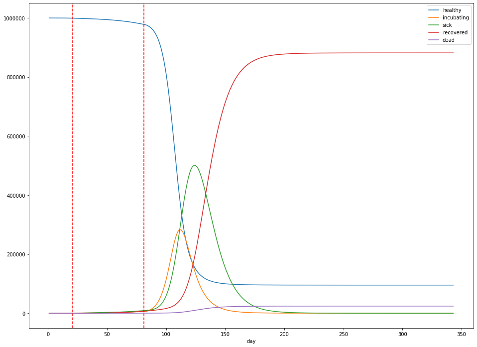
Let’s suppose instead, we institute social distancing with a 2 months on, 1 month off cadence as explored in the ICL paper:

Simulation 5

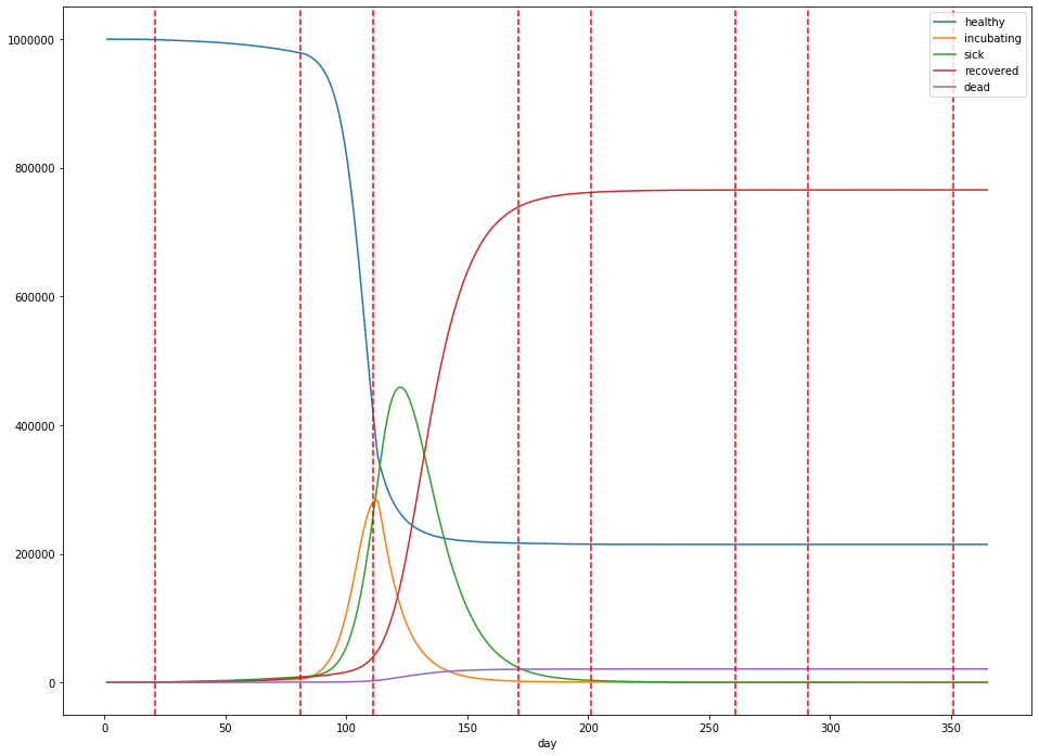
In our simulated world, this delays the eventual peak from 70 days to about 120 days in, but only slightly dampens the height of the peak: about 45.9% of the population is infected at the peak, and the total dead is about 2.1%. Additionally, a total of 765,654 (77%) people are infected over the lifetime of the outbreak.

Finally, let’s do one more simulation—this time, where social distancing is lifted when the rate of new cases slows to zero new cases a day, and the total number of sick people is below 20% of the population. Social distancing is re-instituted when there are more than 1,000 new cases a day.

Simulation 6

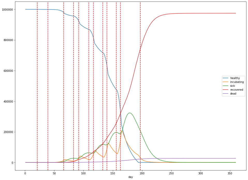
In this case, at its peak, 119,669 people are sick with the virus 200 days into the simulation. The total mortality rate remains stubbornly consistent, with 20,409 dead after 360 days. The lockdowns are imposed from days 21 to 156, days 163 to 180, and days 190 to 201, with the largest peak in infections occuring during the last lockdown. Overall, 739,714 people catch the virus.

Concluding thoughts

This simulation approach is overly simplistic, and obviously gets a few things wrong. To start, every simplifying assumption is likely false. Another possibly less obvious error is that the model is rather pessimistic about the total number of infections (usually in the neighborhood of 75% of the population). Even the most pessimistic forecasts generally don’t go this high. I am not an epidemiologist, but I suspect that one potential source of error is that more sophisticated simulations do not assume homogenous mixing of the population, i.e. that every person in the population may potentially interact with any other in a uniform way. It’s possible that a graph-theoretic approach (simulate a random graph of the connections within the population, and allow the virus to propogate out from one of the nodes) may be more suitable, and can also better model social distancing via pruning of edges of the graph. (In particular, even starting from a connected graph, this approach would eventually lead to a a graph with multiple disjoint components.)

All that being said, this exercise did leave me with a few conclusions:

$R_0$ matters a lot: the more we can do to reduce the probability of passing along the virus, even if you’re not in an at-risk population yourself, the fewer overall deaths we’ll see.
Lockdown directives can lower the peak infection number and delay the peak, but only while they’re in place. It’s likely that lifting any shelter-in-place or lockdown directives will lead to a resurgence in the virus.
The overall number of deaths due to the virus is relatively unaffected by part-time social distancing measures. To reduce fatalities, we must directly lower $R_0$, for a prolonged period of time at likely significant social cost, or change the CFR. This suggests to me that the most effective way to reduce the number of deaths is through better treatment (e.g. antiviral medication or a vaccine), rather than social measures.

Finally, it’s clear to me that we’re in this for the long haul. Anyone who thinks that come April 1st or even April 30th, the lockdowns can be lifted and the virus will just disappear is kidding themselves. At this point, to limit the overall number of deaths, we are engaged in a delaying action: we must slow the spread of the virus to buy enough time for effective treatment options to become available. With luck, some previously developed antivirals will prove effective in the shorter term, and a vaccine will become available in the next 12 months.