Semantic search and short topic models
What is the topic of a sentence? Is this text relevant to a given search term? These are some of the sorts of questions at the heart of search, and whole companies have been built on them. In this post, I’ll look at a very easy way to identify topics of sentences and statements using off-the-shelf libraries (specifically, ExplosionAI’s Spacy and HuggingFace’s NeuralCoref models). We’ll specifically explore two problems: finding all sentences relating to a particular search term or query, and determining a given sentence’s topic.
First, let’s look at query matching. In its simplest form, query matching can be done by looking for specific mentions of a given term within a statement (e.g. via regular expressions). I’d like to do something more clever here (but only slightly so): we can take advantage of word embeddings to find “semantically similar” words to the query terms, and we can also do coreference resolution to identify implicit references to the query term.
A quick recap on word embeddings
To make text usable in most machine learning algorithms, we need to perform tokenization and vectorization. Tokenization is just identifying the tokens that make up the corpus of text (in this case, we’ll use words, but character tokenizations as well as n-gram tokenizations are not uncommon). Vetorization is the process of mapping those tokens to the elements of some vector space.
A completely naive way to accomplish both steps is to tokenize by splitting text on whitespace (i.e. mapping the sentence "It was a great party!" to ["It", "was", "a", "great", "party!"]), and then one-hot encoding the tokens.
Thus, if the entire corpus consisted only of the five tokens in that single sentence, we would end up with embeddings like
"It" --> [1, 0, 0, 0, 0]
"was" --> [0, 1, 0, 0, 0]
"a" --> [0, 0, 1, 0, 0]
"great" --> [0, 0, 0, 1, 0]
"party!" --> [0, 0, 0, 0, 1]
You could clean this up a bit by dropping punctuation and forcing all text to lowercase. Further clean-up steps often include lemmatizing the text (dropping conjugation, declension, etc.) as well as (depending on the use case) eliminating stop words.
However, this kind of vectorization is completely ignorant of the semantic content (that is, the meaning) of the tokens themselves; nouns like “party” are treated identically to verbs and adjectives. It has the additional disadvantage of producing highly sparse embeddings (in the sense that a token’s vector consists primarily of zeroes). These embeddings are also high-dimensional, making them difficult to work with in most traditional machine leanring applications.
I’ll describe one embedding technique that slightly improves on this, which will be relevant for the second part of this post: term frequency inverse document frequency (TF-IDF) embeddings. The idea behind TF-IDF is, for a given corpus of documents (here, document is used loosely to mean any collection of text), we can assign a real number to each word based on how frequently that word appears in a given document (the term frequency) normalized by the number of documents containing that word relative to the overall number of documents. Mathematically, this is:
\[tfidf(t, d, D) := f_{t,d}\cdot \log \left( \frac{|D|}{|\{ d \in D : t \in d \}} \right)\]where $t$ is the term in question, $d$ is the given document, and $D$ is the collection of all documents.
This gives a $|D|$-dimensional embedding of each token (where $t_{k} = 0$ if $t \not{\in} d_{k}$ ). Compared to the naive one-hot embedding, this type of embedding does not have the dimensionality embedding, and for a given document, the spherical mean (the “mean direction”) of all of the tokens in the document is a rough proxy for document topic.
However, TF-IDF still suffers from the deficiency that the word embeddings learned do not necessarily have anything to do with the semantic content of the word. That is, words with similar meanings will not necessarily have similar embeddings. So, how can we construct an embedding that does capture this semantic content?
One idea is the “distributional hypothesis.” This is the linguistic claim that words that are used in similar ways or appear in similar contexts tend to have similar meanings. The context of a word is determined by the words that appear before and after it. So, the distributional hypothesis suggests that a good proxy for the semantic content of a word is the statistical distribution of words that appear nearby. This is the foundational idea behind word embedding schemes like Word2Vec and its relatives (GloVe, BERT, etc). And it turns out to work pretty well—here’s a projection of the word embeddings onto the first two principal components for some “gendered” nouns (man, woman, king, queen, etc) from GloVe:
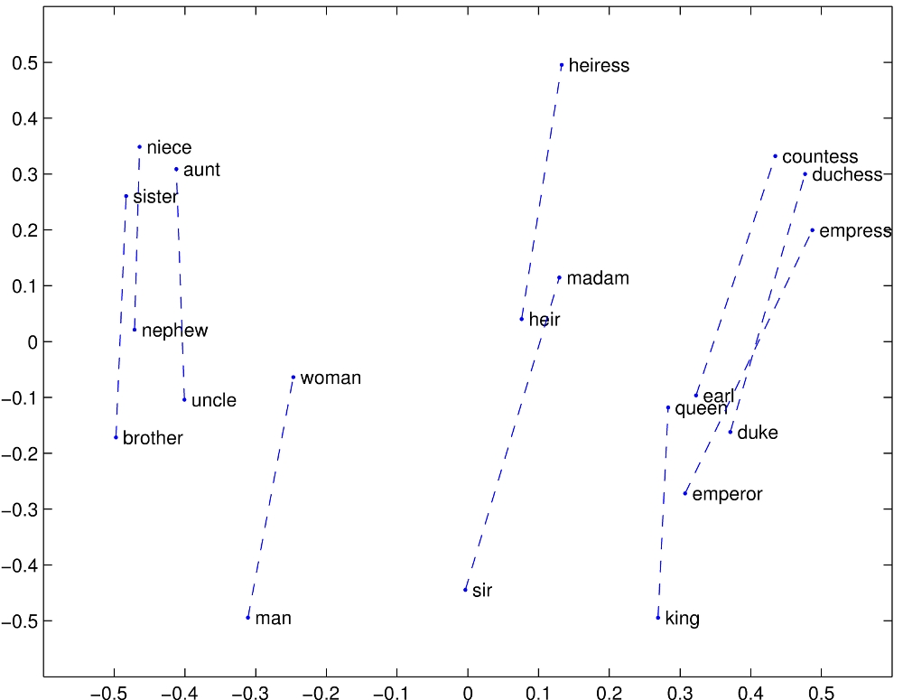
An indication that this approach is actually capturing something semantic about the word content is that we can recover analogies from it. For example,
vec("king") - vec("man") + vec("woman") ~ vec("queen")
(That is, the word vector for “queen” is closest to the word vector you get by subtacting “man” from “king” and adding “woman.” This can be equivalently written as
vec("king") - vec("man") ~ vec("queen") - vec("woman")
which is exactly the type of analogy questions that commonly show up in elementary school English classes:
Man:King :: Woman:Queen
(See nlp.stanford.edu/projects/glove for more.) Word2Vec is well-studied, and any further exposition I’d put here would just be parroting other explanations—for a good reference, check out Jurafsky and Martin’s book.
Finding all sentences relating to a particular term
Let’s take advantage of our newfound understanding of word embeddings to find mentions of the term we’re interested in. As a sample document, I’ll use the raw text of the Wikipedia page for Chicago (see https://en.wikipedia.org/wiki/Chicago). Spacy makes this super easy.
First, let’s set up our pipeline:
import spacy
import neuralcoref
import numpy as np
import pandas as pd

nlp = spacy.load("en_core_web_md")
neuralcoref.add_to_pipe(nlp)
Next, process the document (depending on your machine, this might take a little while; rawtext is the variable I used for the raw string of Wikipedia text).
doc = nlp(rawtext)
Finding sentences containing exact mentions of the search term is easy:
# find match in a specific sentence
def find_exact_match(sentence, term):
    if term.lower() in sentence.text.lower():
        yield sentence

# find all matches in the document
def find_exact_matches(doc, term):
    for sent in doc.sents:
        for match in find_exact_match(sent, term):
            yield match

[_ for _ in find_exact_matches(doc, "Urbs in Horto")]
# Produces the output
# ['When Chicago was incorporated in 1837,
#   it chose the motto Urbs in Horto, a Latin phrase
#   which means "City in a Garden".']
Note that the construction here is a chain of iterators; the functools module in the standard library could be used to make the presentation a little cleaner.
Sprucing up the find_exact_match function to incorporate vector similarity is straightforward.
The token vectors can be found with the .vector attribute, and cosine similarity is used for determining word similarity.
(Note that Spacy includes a built-in token similarity function—token.similarity()—which is just the cosine distance under the hood.
We’ll be modifying our token vectors for sentence topics later on, so I’ve written it out explicitly here.)
def dist(v1, v2):
    return np.dot(v1, v2)/(np.linalg.norm(v1)*np.linalg.norm(v2))

def find_sim_match(sentence, term, thresh=0.7):
    v1 = term.vector
    for token in sentence:
        if dist(v1, token.vector) > thresh:
            yield sentence
            return

def find_sim_matches(doc, term, thresh=0.7):
    term = nlp(term)
    for sent in doc.sents:
        for match in find_sim_match(sent, term, thresh):
            yield match
Comparing this against our exact matches, we see that this turns up some additional relevant sentences:
[_ for _ in find_matches(doc, "medicine")][0]
# Returns:
# "The Chicago campus of Northwestern University includes
#  the Feinberg School of Medicine; Northwestern Memorial
#  Hospital, which is ranked as the best hospital in the
#  Chicago metropolitan area by U.S. News & World Report for
#  2017–18;[326] the Shirley Ryan AbilityLab (formerly
#  named the Rehabilitation Institute of Chicago), which
#  is ranked the best U.S. rehabilitation hospital by U.S.
#  News & World Report;[327] the new Prentice Women's Hospital;
#  and Ann & Robert H. Lurie Children's Hospital of Chicago."

[_ for _ in find_sim_matches(doc, "medicine")][0]
# Returns:
# "City, and later, state laws that upgraded standards for
#  the medical profession and fought urban epidemics of cholera,
#  smallpox, and yellow fever were both passed and enforced."
In the second case, our search is finding sentences that contain related words to medicine (e.g. “medical”), even though the search term itself does not explicitly appear.
(Some tuning is required to determine exactly how broad the search can be—the threshold of 0.7 corresponds to an angle of about 45 degrees between the two word vectors.)
Adding coreferences
Next let’s take a look at how to further improve our search by adding coreferences. For illustrative purposes, let’s first consider HuggingFace’s example text:
My sister is swimming with her classmates. They are not bad, but she is better.
I love watching her swim.
(The linked text shows an illustration of how the coreference detection works.) Finding the coreferences is straightforward:
ex_doc = nlp(ex_string)

for token in ex_doc:
    clusters = token._.coref_clusters
    for c in clusters:
        if token not in c.main:
            print("{} --> {}".format(token, c.main))
# output:
her --> My sister
They --> her classmates
she --> My sister
her --> My sister
The neuralcoref package adds coreference clusters to any span in the text containing a potential coreference.
The coreference clusters have a main attribute, indicating the “referant” term.
Checking that the token is not part of the main reference filters the primary reference (which would otherwise also appear in our coreference check).
Let’s add this to our matching function:
def dist(v1, v2):
    return np.dot(v1, v2)/(np.linalg.norm(v1)*np.linalg.norm(v2))

def find_coref_sim_match(sentence, term, thresh=0.8):
    v1 = term.vector
    for token in sentence:
        if dist(v1, token.vector) > thresh:
            yield sentence
            return
        clusters = token._.coref_clusters
        for c in clusters:
            if token not in c.main:
                if dist(v1, c.main.vector) > thresh:
                    yield sentence
                    return

def find_coref_sim_matches(doc, term, thresh=0.7):
    term = nlp(term)
    for sent in doc.sents:
        for match in find_coref_sim_match(sent, term, thresh):
            yield match
As a quick check that this is working, let’s look at a simple example:
ex_doc = nlp('''John had a dog. It was named Max.''')
[_ for _ in find_coref_sim_matches(ex_doc, "dog")]
# Returns
# [John had a dog., It was named Max.]
Our previous technique only picks up the first sentence:
[_ for _ in find_sim_matches(ex_doc, "dog")]
# Returns
# [John had a dog.]
Note that neuralcoref is not perfect: some coreferences are missed or difficult for it to resolve.
Also, the incidence of coreferences will depend on the author and the type of text (for example, formal encyclopediac writing, such as Wikipedia articles, may have fewer coreferences to avoid ambiguity).
Topic models
Now that we have the ability to identify sentences containing content relevant to a given search term, we’ll look at the dual problem: given a sentence, what is that sentence about? As before, the answer will hinge on vector embeddings of words.
The basic idea is the following:
- For each sentence, compute some “weighted aggregate” word vector.
- Identify the sentence’s topic by finding the word in our vocabulary whose word vector is closest to the sentence’s weighted aggregate word vector.
For part 1, the naive approach would be to assign each sentence the average of the word vectors for each token in the sentence. However, this approach weights each word equally, which might not be what we want: the indicator of the sentence’s topic may only appear once, relative to the other text. Fortunately, we have a tool for weighting tokens based on rarity: TF-IDF. In particular, let’s compute TF-IDF scores for tokens by considering each sentence as a “document” and the document as a whole as our corpus. This computation can be done by adding a TF-IDF function to our Spacy pipeline:
from spacy.lang.en import STOP_WORDS
from spacy.tokens import Token

# tf-idf weightings
Token.set_extension("tfidf", default=0.0)

def compute_tfidf(doc):
    sents = [_ for _ in doc.sents]
    n = len(sents)
    freqs = {}
    for sent in sents:
        tokens = set()
        for token in sent:
            if token.text in STOP_WORDS or token.is_punct:
                continue
            if token.lemma_ in tokens:
                continue
            tokens.add(token.lemma_)
            if token.lemma_ in freqs:
                freqs[token.lemma_] += 1
            else:
                freqs[token.lemma_] = 1
    for lemma in freqs:
        freqs[lemma] = math.log(n/(1.0 + freqs[lemma]))
    for token in doc:
        if token.lemma_ in freqs:
            token._.tfidf = freqs[token.lemma_]

    return doc

#tfidf calc
nlp.add_pipe(compute_tfidf, name="tfidfer", last=True)
Next, we can wrap this up into a function to compute our TF-IDF-weighted topic vector:
def compute_topic_vector(sentence):
    vector = np.zeros(300) # vectors are size 300
    for token in sentence:
        if token.text in STOP_WORDS:
            clusters = token._.coref_clusters
            for c in clusters:
                if token not in c.main:
                    count = len([t for t in c.main if t not in STOP_WORDS])
                    for token2 in c.main:
                        vector = vector + token2._.tfidf*token2.vector/count
        else:
            vector = vector + token._.tfidf*token.vector
    vector = np.divide(vector, len(sentence))
    return vector
The function above also reuses portions of our coreference resolution code so that we’ll correctly detect sentence topics even if the topic itself does not explicitly appear. Also, stop words are explicitly being ignored in both our TF-IDF computation as well as the topic vector computation.
Finally, once we have a topic vector, how do we find the token closest to that topic? There are two ways to think about approaching this problem: we can either try to identify the topic from a pre-determined list of topics, or we can try to identify the topic by selecting the word in our vocabulary that is closest to the topic vector we constructed. The first approach can be readily accomplished by re-using our distance code from the first part of this post. For the second, we could conceivably loop through every word in the vocabulary and also compute the distance. Doing this in pure Python is likely to be slow, however, and Spacy has some under-the-hood (and somewhat lightly documented) functionality to let us do this. (Spacy isn’t really designed for this kind of thing; libraries like Gensim have this functionality built in out of the box.)
Here’s our function:
def nearest_vector(doc, vector):
    idx = doc.vocab.vectors.most_similar(vector.reshape(1,-1))[0][0]
    return doc.vocab[idx].text.lower()
This returns the text of the lexeme, which may not be exactly what one expects. For example,
nearest_vector(nlp("camera"), nlp("camera").vector)
# returns "videocamera"

nearest_vector(nlp("bank"), nlp("bank").vector)
# returns "citibank"
Putting it all together, here are the topics we infer for the first 10 sentences in the Chicago Wikipedia article:
counter = 0

for sentence in doc.sents:
    counter += 1
    vec = compute_topic_vector(sentence)
    topic = nearest_vector(doc, vec)
    print("{}. {}\n--> {}\n".format(counter, sentence, topic))
    if counter > 10:
        break
1. Chicago, officially the City of Chicago, is the most populous city
in the U.S. state of Illinois and the third most populous city in
the United States.
--> metropolis

2. With an estimated population of 2,705,994 (2018), it is also the
most populous city in the Midwestern United States.
--> population

3. Chicago is the county seat of Cook County, the second most populous
county in the US, with portions of the northwest city limits extending
into DuPage County near O'Hare Airport.
--> township

4. Chicago is the principal city of the Chicago metropolitan area,
often referred to as Chicagoland.
--> metropolis

5. At nearly 10 million people, the metropolitan area is the third most
populous in the nation.
--> surpassed

6. Located on the shores of freshwater Lake Michigan, Chicago was incorporated
as a city in 1837 near a portage between the Great Lakes and the Mississippi
River watershed and grew rapidly in the mid-19th century.[7]
--> lakeside

7. After the Great Chicago Fire of 1871, which destroyed several square miles
and left more than 100,000 homeless, the city made a concerted effort to
rebuild.[8]
--> surpassed

8. The construction boom accelerated population growth throughout the following
decades, and by 1900, less than 30 years after the great fire, Chicago was the
fifth-largest city in the world.[9]
--> half-century

9. Chicago made noted contributions to urban planning and zoning standards,
including new construction styles (including the Chicago School of architecture),
the development of the City Beautiful Movement, and the steel-framed
skyscraper.[10][11]

Chicago is an international hub for finance, culture, commerce, industry,
education, technology, telecommunications, and transportation.
--> developement

10. It is the site of the creation of the first standardized futures contracts,
issued by the Chicago Board of Trade, which today is the largest and most
diverse derivatives market in the world, generating 20% of all volume in
commodities and financial futures
--> market
Qualitatively, these topic assignments seem reasonable! Observe that Spacy’s sentencizer struggles with statement 9 (which is actually two sentences); this is likely because of the citations. This post just scratches the surface of what’s possible, and there’s ample room for tuning. For example:
- If all text is domain-specific, training word embeddings on a domain-specific corpus will lead to more granular topic modeling and potentially better term matching performance.
- Spacy’s dependency parsing can be used to improve the topic vector choice (e.g. by taking into account parts of speech).