Exponential smoothing like a Bayesian

Written on April 12, 2022

Exponential smoothing is a class of forecasting methods in which weighted averages of past observations are used to predict future values. Exponential smoothing is particularly popular for financial time series because, unlike many other forecasting methods (e.g. ARIMA models), exponential smoothing does not require the underlying series to be stationary (or stationary after differencing). However, many financial time series (such as stock prices) are highly noisy, and exponential smoothing models have to be fit recurrently, using numerical optimization. After fitting, how can we construct confidence intervals for the parameters of our exponential smoothing model? In this post, I’ll describe one way to attack this problem using probabilistic programming, and provide examples using Julia’s Turing package.

This post is divided into three parts: First, I’ll give a quick overview of exponential smoothing. Next, we’ll look at the problem of parameter estimation for exponential smoothing models, and motivate why we should consider taking a Bayesian approach here. Finally, I’ll show how to fit an exponential smoothing model using Bayesian probabilistic programming, and I’ll describe how this can be used as a test for momentum and mean-reversion in time series. At the very end, we’ll apply this methodology to a real financial time series (closing prices of SPY).

What is exponential smoothing, anyway?

Exponential smoothing describes a class of models where the next forecast is constructed from weighted averages of the previous observations. This is similar to a moving average except that, rather than using uniform weights, the weights decay (exponentially) with the age of the observation.

The simplest exponential smoothing model only has one parameter, $\alpha \in [0, 1]$, and has the following form:

\[\hat{y}_{t+1}=\alpha y_{t}+(1-\alpha)\hat{y}_{t}\]

where $\hat{y}_{t}$ is the predicted value of the series at time $t$. The parameter $\alpha$ determines how quickly the contribution of prior observations “decays”: let $l_0 := \hat{y}_0$, then this expression expands to

\[\hat{y}_{t+1}=\sum_{k=0}^{t-1}\alpha(1-\alpha)^{k}y_{t-k}+(1-\alpha)^{t}l_{0}\]

and in particular, $\alpha (1 - \alpha)^{k} y_{t-k}$ is the coefficient of the $k$ th lagged observation.

Introducing trends to exponential smoothing

The simple exponential smoothing above only accurately describes time series that exhibit a kind of mean reversion (strong movement in one direction will tend to be followed by movement in the opposite direction). This can be seen explicitly by re-writing the exponential smoothing model in “component” form:

If we call \(l_{t} := \hat{y}_{t}\) the level we can re-write exponential smoothing as:

\[\hat{y}_{t+1} = l_{t}\] \[l_{t} = \alpha y_{t} + (1 - \alpha) l_{t-1}\]

The first equation is often called the forecast rule, and the second equation the update rule. The update rule can be re-written as:

\[l_t = l_{t - 1} + \alpha (y_{t} - l_{t-1})\] \[= l_{t - 1} + \alpha \varepsilon_{t}\]

where \(\varepsilon_{t} := y_{t} - \hat{y}_{t}\) is the residual at time $t$.

This is a state space formulation of exponential smoothing: $l_{t}$ is the state of the series at time $t$, and the equation \(y_{t+1} = l_{t} + \varepsilon_{t + 1}\) is a function that maps the state to a forecast for the next observed value. (You may notice that this state space formulation is reminiscent of recurrent neural networks, and indeed many types of time series models—including ARIMAs and RNNs—have a state space formulation.)

For our purposes, one advantage of the state space formulation is that trend can be incorporated into the model in a very natural way. Let’s denote the trend at time $t$ by $b_t$ (a real number). How might we add some trend to our forecast? The obvious thing to do is just add it:

\[y_{t} = l_{t - 1} + b_{t - 1} + \varepsilon_{t}\]

But now, $b_t$ is a part of the state of our model, so we should update it as well. Just like the level is a weighted average of previous observations, so too should the trend be a weighted average of the previous slopes of the series. Thus we arrive at Holt’s linear trend formulation of exponential smoothing:

\[y_{t} = l_{t-1} + b_{t - 1} + \varepsilon_{t}\] \[l_{t} = l_{t - 1} + b_{t - 1} + \alpha \varepsilon_{t}\] \[b_{t} = b_{t - 1} + \alpha \beta \varepsilon_{t}\]

where $\beta \in [0, 1]$ is a parameter controlling the decay of the slope over time.

In practice, this linear trend can lead to inaccurate forecasts: a forecast $k$ steps ahead is given by

\[\hat{y}_{t+k} = l_{t} + k b_{t}\]

so in this model the current trend continues indefinitely into the future. To combat this, a damping factor $\phi \in [0, 1]$ is introduced into the model. This produces an additive damped trend exponential smoothing model:

\[y_{t} = l_{t - 1} + \phi b_{t-1} + \varepsilon_{t}\] \[l_{t} = l_{t - 1} + \phi b_{t - 1} + \alpha \varepsilon_{t}\] \[b_{t} = \phi b_{t - 1} + \alpha \beta \varepsilon_{t}\]

If you’re familiar with ARIMA models, this formulation is equivalent to an ARIMA(1,1,2) model, where $\phi_{1} = \phi$, $\theta_{1} = \alpha + \phi \alpha \beta - 1 - \phi$, and $\theta_{2} = (1 - \alpha) \phi$.

Some examples of exponential smoothing

Below are three examples of exponential smoothing models, for different choices of $\alpha$, $\beta$, and $\phi$. In each case the noise is standard Gaussian: $\varepsilon \sim \mathcal{N}(0, 1)$.

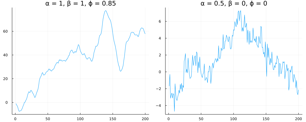
First, a pure arithmetic random walk: $\alpha = 1$ and $\beta = \phi = 0$

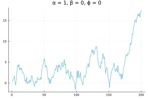
There is nothing predictable about this series. But now suppose we decrease $\alpha$:

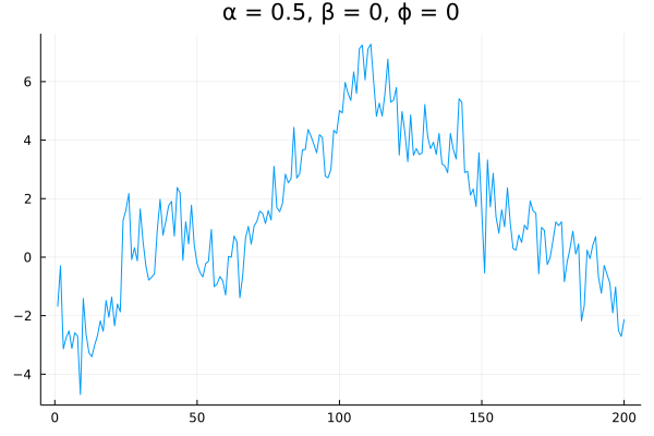
The series exhibits clear mean reversion—a step in any one direction is likely to be followed by a step in the opposite direction. The closer $\alpha$ is to zero, the more this series will resemble Gaussian noise centered at 0.

Finally, let’s set $\alpha = 1$ like in our random walk example, but crank up $\beta$ and $\phi$:

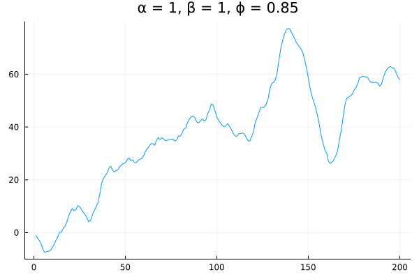
Note that I’ve set $\phi = 0.85$ instead of $1$ so that the trends decay more quickly. This series clearly exhibits momentum: movement in one direction is very often followed by movement in that same direction.

Confidence intervals for model parameters

When it comes to how we would fit an exponential smoothing model, up until this point I’ve just gestured vaguely at numerical optimization. Most numerical optimization techniques (e.g. gradient descent) don’t come out of the box with any confidence intervals for the best-fit parameters they return. On the other hand, we do have confidence intervals for certain types of time series models, so why is this problem hard for exponential smoothing?

Let’s first review how you get confidence intervals in ordinary least squares (OLS) regression problems. We can use OLS to solve for autoregressive (AR) models, such as an AR(2) model. The “2” just means we’re including 2 lagged terms, e.g. the model looks like:

\[y_t = \phi_{1} y_{t-1} + \phi_{2} y_{t-2}\]

The least-squares best fit values for the parameters $\phi_{1}$ and $\phi_{2}$ can be found explicitly: we have the system of equations

\[\underbrace{\left[\begin{matrix}y_{3}\\ y_{4}\\ \vdots\\ y_{n} \end{matrix}\right]}_{=Y}=\underbrace{\left[\begin{matrix}y_{2} & y_{1}\\ y_{3} & y_{2}\\ \vdots & \vdots\\ y_{n-1} & y_{n-2} \end{matrix}\right]}_{=X}\underbrace{\left[\begin{matrix}\phi_{1}\\ \phi_{2} \end{matrix}\right]}_{=\beta}\]

and the optimal $\beta$ is given by

\[\beta_{opt} = (X^T X)^{-1} X^T Y\]

To find the confidence intervals, we write

\[Y \sim X \beta_{true} + \varepsilon\]

where $\beta_{true}$ represents the “true” weights, and $\varepsilon \sim \mathcal{N}(0, \eta^2 I)$ is an $n-2$-dimensional multivariate Gaussian distribution representing the noise the noise for each residual (which is assumed to be uncorrelated and identically distributed with variance $\eta^2$).

Since $Y \sim \mathcal{N} (X \beta_{true}, \eta^2 I)$ and $\beta_{opt} = (X^T X)^{-1} X^T Y$ is a linear transformation of $Y$, we can apply the linear transformation to this expression:

\[\beta_{opt} := (X^T X)^{-1} X^T Y\] \[\sim \mathcal{N} ( (X^T X)^{-1} X^T X \beta_{true}, ((X^T X)^{-1} X^T) \eta^2 I ((X^T X)^{-1} X^T)^T )\]

which, after some simplification, becomes

\[\beta_{opt} \sim \mathcal{N}( \beta_{true}, \eta^2 (X^T X)^{-1} )\]

(Wei Yi has a longer derivation of this here.). $\eta^2$ can be estimated from the variance of the residuals, and our best estimate of $\beta_{true}$ is $\beta_{opt}$. From this expression, we can extract confidence intervals for each coefficient.

The point of this digression is that confidence intervals from OLS regression are a lucky consequence of the analytic solution for $\beta_{opt}$ ! The exercise above breaks down as soon as the model solution can’t be expressed as an OLS problem, which happens immediately for our exponential smoothing models.

So what do we do? It’s time to get Bayesian.

Bayesian modeling

Bayesian modeling starts from Bayes’ rule:

\[P(\theta|E)=\frac{P(E|\theta)P(\theta)}{P(E)}\]

In contrast to the common expression in terms of generic events $A$ and $B$, I’ve written it suggestively with variables $\theta$ and $E$. This is to promote following interpretation of Bayes rule: the probability of the model $\theta$ given the evidence $E$ is equal to the probability of the evidence given the model, multiplied by the prior probability of the model, and divided by the probability of the evidence. This interpretation is important enough that each term in Bayes’ rule gets a name:

• The term \(P(\theta \mid E)\) is called the posterior distribution of the model parameter, and represents how we should update our model given the available evidence (this is the distribution we want to discover);
• The term \(P(E \mid \theta)\) is called the likelihood distribution, and represents how likely this data would be to occur given our prior model;
• The term \(P(\theta)\) is called the prior distribution, and represents our estimate of the model parameters prior to seeing any data;
• The term \(P(E)\) is called the marginal distribution, and is the likelihood of the data averaged across all possible models.

If you haven’t seen this stuff before, it can be confusing, so let’s look at an example.

The Bayesian “hello world” example

Imagine we have a weighted coin that, unbeknownst to us, has a 75% chance of producing heads when we flip it. Suppose the coin is flipped 10 times. Perhaps the flips are

1.  heads
2.  heads
3.  tails
4.  heads
5.  tails
6.  heads
7.  heads
8.  heads
9.  tails
10. heads

A simple model for this coin flip is that $P(H) = \theta$ and $P(T) = 1 - \theta$. This model has a single parameter, $\theta$, representing the probability of heads. Our goal is to figure out what the most likely value of $\theta$ is, given our observed flips. Going into this experiment, we have no knowledge of whether the coin is fair or not, so we choose as a prior the $\beta(1, 1)$ distribution (uniform probability = 1 on the interval [0, 1]; 0 elsewhere).

With each flip, we can apply Bayes’ rule to compute our updated posterior distribution for $\theta$:

The choice of the Beta distribution is important here because the Beta distribution is the conjugate prior to the Bernoulli distribution (which describes the coin flips), meaning that Bayes’ rule actually has an analytic solution for the posterior.

In particular,

\[P(E|\theta) = \theta^{k} (1 - \theta)^{n - k}\]

where $k$ is the number of heads observed and $n$ the total number of tosses, and

\[\beta(\alpha, \beta)(\theta) = \frac{\theta^{\alpha - 1} (1 - \theta)^{\beta - 1}}{B(\alpha, \beta)};\]

hence

\[P(\theta | E) = \frac{\theta^{k}(1 - \theta)^{n-k} \beta(1, 1)}{P(E)}\]

which is readily verified to be a Beta distribution.

For the rest of this post, we will not be so lucky—most of the time, there will be no analytic solution for $P(\theta | E)$. So what do we do?

Markov Chain-Monte Carlo

Fortunately, we are not completely out of luck. A family of techniques called Markov Chain-Monte Carlo (MCMC) methods allow us to sample from a probability distribution, even if we can’t write it out explicitly. The simplest example of this is the Metropolis algorithm, which I will attempt to summarize here.

The primary advantage of the Metropolis-Hastings algorithm is that we only need a function that is proportional to the desired probability density function to draw samples from it, rather than exactly equal. This exactly describes the situation we’re in: often we can draw samples from our prior distribution $P(\theta)$ as well as from our likelihood distribution $P(E \mid \theta)$, but computing the normalization is typically difficult.

Here is the algorithm:

Suppose that $f(x)$ is a function proportional to the distribution we want to draw samples from, and $g(x|y)$ is an arbitrary probability density function (e.g. a Gaussian distribution centered at y). Initialize by picking an arbitrary point $x_0$ to be the first observation in the sample. Then, for each iteration:

1. Select a candidate for the next point $x’$ by sampling from the distribution $g(x’ \mid x_{t})$
2. Calculate the acceptance ratio $\lambda = f(x’) / f(x_t)$
3. Pick a uniform random number $u \in [0, 1]$; if $u \leq \lambda$ then accept the candidate by setting $x_{t+1} = x’$, otherwise reject the candidate and set $x_{t+1} = x_{t}$ instead.

The intuition is that, if $x’$ is more probable than $x_{t}$, the algorithm will always advance to $x’$, but if $x’$ is less probable than $x_{t}$, the algorithm may choose to stay put. Over time, this will result in a large number of samples from the higher-density regions of $P(X)$, and fewer samples from low-density regions of $P(X)$.

This allows us to draw samples from the posterior distribution without needing to write an analytic solution for it. Note, however, that the Metropolis algorithm has some disadvantages: individual samples are correlated with each other, so there is often a “burn in” period needed before the chain of samples resembles the desired distribution. More advanced variations on this algorithm like Hamiltonian Monte Carlo (HMC) sampling partly address this deficiency.

Enough theory, let’s just get to the code part

The MCMC or HMC techniques mentioned above form the foundation for a class of tools called probabilistic programming languages. There are many great examples of these: the most famous is Stan (which probably has bindings to your favorite language), and there’s also PyMC3 and Pyro for Python. I’ve become something of a Julia stan lately, though, so in this post we’ll be using Julia’s Turing package.

If you’d like to follow along and haven’t used Turing before, you’ll need to add the following packages to your Julia environment: Statistics, Turing, Distributions, and StatsPlots. All of these can be added with ] add <packagename> from the Julia REPL.

Next, we need to specify our model. Turing adds the @model macro to make this easy:

@model function ets(y)

    # priors for the model parameters
    α ~ Beta(1, 1)
    β ~ Beta(1, 1)
    ϕ ~ truncated(Beta(1, 1), 0.7, 1.0)
    σ2 ~ truncated(Normal(0, 1), 0, Inf) # variance
    l ~ Normal(y[1], 1) # initial level
    b ~ Normal(0, 1)    # initial trend

    for i = 1:length(y)
        ŷ = l + ϕ * b # forecast
        y[i] ~ ŷ + Normal(0, sqrt(σ2)) # observation

        ε = y[i] - ŷ # forecast error
        l = l + ϕ * b + α * ε # update the level
        b = ϕ * b + α * β * ε # update the trend
    end
end

The first part of this function specifies the priors we’re choosing for the model parameters. In particular, I’ve chosen noninformative priors for most of the model parameters: the only thing I know about $\alpha$, $\beta$, and $\phi$ is that they should all be between 0 and 1, and the only thing I know about $\sigma^2$ (the variance of the error) is that it is greater than zero. (In fact, I have constrained $\phi$ to be between 0.7 and 1 because in practice it is difficult to distinguish between small $\phi$ and small $\beta$.) I have additionally guessed that the initial level $l_0$ is most likely equal to the first observation $y_1$, and that the initial trend is most likely zero.

The for loop in this function then computes the likelihood function of each observation, given our model parameters:

ŷ = l + ϕ * b
y[i] ~ ŷ + Normal(0, sqrt(σ2))

and the error ε = y[i] - ŷ is used to update the state of the model.

We now have what we need to apply this to some actual data.

Example 1: a pure arithmetic random walk

Let’s first apply it to our pure random walk ($\alpha = 1$, $\beta = \phi = 0$) from above:

We’ll use the no-U-turn sampler (NUTS), an advanced HMC sampler, to estimate the posterior distributions on our various model parameters, given these observations. This can be done by calling Turing’s sample function:

chain = sample(ets(random_walk), NUTS(), 5_000)

(where random_walk is an array containing the observed values of the time series, NUTS() is the default argument NUTS sampler, and I am using 5,000 iterations for my sampling.) We can get a summary of the results of the sampling by calling

StatsPlots.plot(chain, fmt=:png)

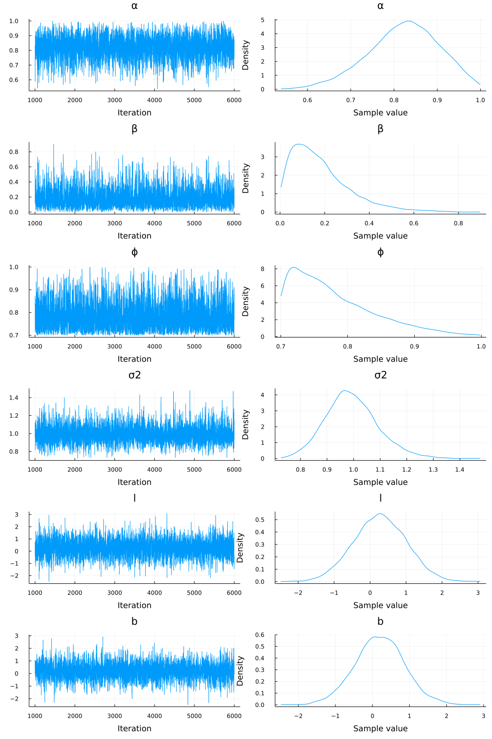
The left-hand column shows the sequence of samples from the chain. This gives us an indication of the quality of our sample: the thing to look for is that there are no clear trends or autocorrelations in the sampled values; each value should look like it has been drawn from the same distribution. The right-hand column of images shows the estimated probability densities for each parameter (based on the generated samples). In particular, the samples suggest that, for the exponential smoothing model that best describes this data, there’s a high probability that $\alpha < 0.9$ and $\beta > 0.1$, which is surprising because we know that the true values used to generate this series were $\alpha = 1, \beta = \phi = 0$.

We can get more precise in assigning probabilities to these possibilities by directly inspecting the samples. For example, to determine the 95% confidence interval for $\alpha$:

> quantile(chain[:α][:,1], 0.025), quantile(chain[:α][:,1], 0.975)
(0.647101, 0.966354)

so with 95% confidence, the value of $\alpha$ for the exponential smoothing model that generated this data is between 0.65 and 0.97. (The [:,1] in chain[:α][:,1] is because the chain object is a $5000 \times 1$ dimensional matrix, where the 1 is because $\alpha$ is a one-dimensional parameter.) Similarly, the 95%-confidence intervals for $\beta$ is $[0.014, 0.52]$ and for $\phi$ it’s $[0.703, 0.935]$.

But wait, you complain—this is not exactly a ringing endorsement of this methodology! The median estimates for these distributions are a ways off, and the confidence intervals are huge! This is for two main reasons:

1. There are many choices of parameters for exponential smoothing models that are “close” to a random walk, e.g. it is difficult to distinguish a model with $\alpha = 0.9$ and $\beta = 0.2$ from one with $\alpha = 1.0$ and $\beta = 0$; and
2. For any given finite sequence, there will always be a choice of exponential smoothing parameters that better fit the data than a pure random walk (because you have 5 additional degrees of freedom: $\alpha$, $\beta$, $\phi$, $l_0$, and $b_0$).

The indication that the above series is likely to be a random walk comes not from the maximum likelihood choice of parameters, but from the very wide confidence intervals on those parameters. We’ll see this more clearly in the next example.

Example 2: Momentum and mean-reverting series

Let’s test it on our momentum (below left) and mean-reverting (below right) series.

First, for the momentum series, I find:

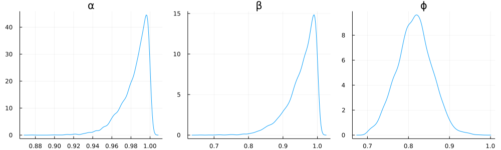
In this case, the 95% confidence intervals are:

• $\alpha$: $[0.947, 1.0]$; median $0.988$
• $\beta$: $[0.845, 1.0]$; median $0.965$
• $\phi$: $[0.732, 0.899]$; median $0.815$

So, in this case, we have much tighter estimates (with medians close to the true values).

Next, the mean-reverting series:

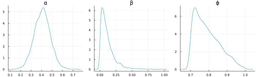
The 95% confidence intervals are:

• $\alpha$: $[0.255, 0.561]$; median $0.408$
• $\beta$: $[0.004, 0.421]$; median $0.084$
• $\phi$: $[0.703, 0.946]$; median $0.778$

Again, we are both more confident and reasonably accurate for $\alpha$ and $\beta$: the true $\alpha$ was 0.5, and the true $\beta$ was 0. But what about $\phi$? This is actually something of a degenerate case for an exponential smoothing model: As $\beta \rightarrow 0$, it becomes difficult to meaningfully estimate $\phi$, and vice-versa; this is why $\phi$ is constrained in our model to lie within 0.7 and 1.0.

Testing on some real data

Now let’s do the test all the quants reading this have been waiting for: applying this to a real financial time series. As in my Hurst exponent post, I’ll use SPY’s historical closing prices (adjusted). You can find this data here. Here is a plot of SPY from December 2017 to April 2022:

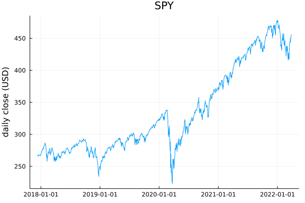
What do you think? Is it mean reverting? Is there momentum? The Hurst exponent test we applied previously suggested very little mean reversion. Let’s check:

chain = sample(ets(spy.Close), NUTS(), 5_000)

Here’s what I find:

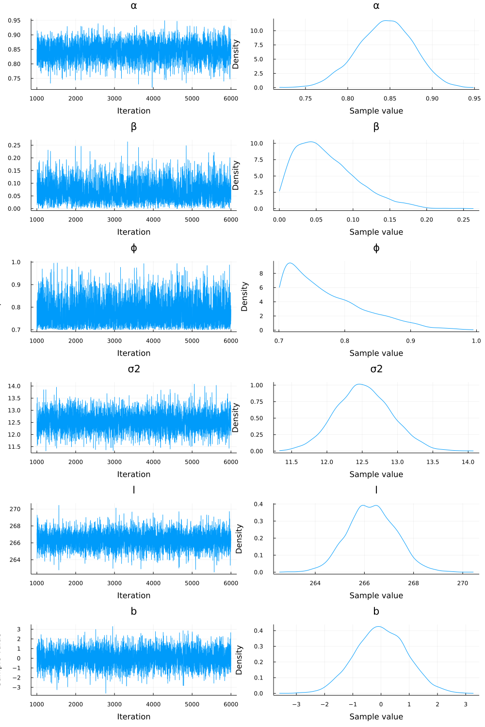
In particular, the 95% confidence range for the model parameters is:

• $\alpha$: $[0.777, 0.906]$ with a median of $0.845$;
• $\beta$: $[0.005, 0.164]$ with a median of $0.056$;
• $\phi$: $[0.702, 0.911]$ with a median of $0.756$

Based on these numbers, I would argue that SPY was weakly mean-reverting during this time period (with a 95% chance that $\alpha < 0.897$), while any momentum effects were comparatively minor (with only an 18.6% chance that $\beta > 0.1$). This is not a particularly surprising result, though: inspecting the plot shows that after the crashes of December 2018, March 2020, and January 2022, SPY reverted back to its previous value relatively quickly. (This does not constitute investing advice!)

Probabilistic programming languages have historically had a reputation for being slow and cumbersome, so here’s one final remark on the practicality of all of this: Running the HMC sampling across about 1000 days of SPY prices to estimate the model parameters took less than 10 seconds on my (boring, consumer-grade) desktop, which is only a couple of seconds longer than it takes Julia’s Optim package to select model parameters via maximum likelihood estimation. This actually makes it one of the more performant parts of my Julia toolbox when doing data analysis.

If your prior belief was that Bayesian inference was impractical or mostly useless, I hope I’ve managed to slightly shift your posterior. And that concludes this post!