Deep learning in low dimensions
Nets work great for problems involving lots of high-dimensional data (such as image or text problems). But, they often struggle for problems with low-dimensional inputs, particularly in cases where the response is not especially smooth with respect to the input. In this post, we’ll explore one way to get around this using “Fourier encodings”, and tackle a couple of interesting applications of this technique, including as a tool for portfolio construction.
Why is low-dimensional data challenging?
To some deep learning proponents, it might seem bold to claim that low-dimensional data challenges nets. By low-dimensional data, I mean problems where the input consists of only a few numeric fields, or where the response is heavily dependent on a single or small number of fields. There’s an intuitive reason why a net might struggle to learn such a response: Nets are differentiable functions, and essentially locally linear (explicitly in the case of ReLU activations). A response that is highly sensitive to slight changes in the input will have strong gradients, and therefore pose challenges to learn (even if, in principle, it should be possible to model it with a net). A toy example of this is the sine function we looked at previously:
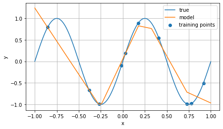
Here, the input is one-dimensional ($x$), and the response is a simple trigonometric function $\sin(x)$. In this case, only a few points were used for training to illustrate the piecewise-linear nature of a feedforward net with ReLU activations. The model struggles particularly to capture a nonlinear relationship in the region between $x=0.5$ and $x=1.0$: three sample points are close together in $x$, but the $y$ value of the third is quite different from the others. When applied to a step function (sampling 1000 points for training), a different problem appears:
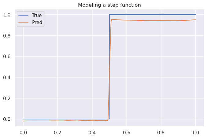
By construction, the model cannot produce a step function, it can only approximate it via piecewise linear functions. This is apparent in the steep but discernable slope near $x = 0.5$. (This net also seems to struggle with points where $y = 1$ and, to a somewhat lesser degree, points where $y = 0$, but it is possible that adding more parameters would address this.)
Unfortunately, outside of NLP and image recognition, many real-world problems involve relatively low-dimensional numeric data. So what is to be done?
Fourier features
In 2020, Tancik et al utilized a Fourier feature construction proposed by Rahimi and Recht to create “positional encodings”, originally for use in neural radiance fields. The approach can be seen as being an extension of the positional encodings proposed in the famous paper “Attention is all you need”. The idea is map an input point $\mathbf{v}$ (such as a pixel coordinate $(x, y)$) to a higher-dimensional space by applying a trigonometric transformation:
\[\gamma(\mathbf{v}) = [\cos (2 \pi \mathbf{B} \mathbf{v}), \sin(2 \pi \mathbf{B} \mathbf{v})]^{\mathrm{T}}\]Here, $B$ is a random Gaussian matrix, that is, a matrix whose elements are randomly sampled from a Gaussian distribution $\mathcal{N}(0, \sigma)$. Varying the scale $\sigma$ controls the Fourier feature frequency, and can be seen as a way of controlling how closely the model fits (underfits, for low $\sigma$, or overfits, for high $\sigma$) the data.
This kind of embedding is quite easy to implement in PyTorch. For example:
import torch
import torch.nn as nn

class FourierEmbedding(nn.Module):

    def __init__(self, in_dim: int, out_dim: int, scale: float = 10):
        super().__init__()
        self.in_dim = in_dim
        self.out_dim = out_dim
        self.B = nn.Parameter(
            scale * torch.randn(in_dim, (out_dim - in_dim) // 2)
        )

    def forward(self, x):
        return torch.cat(
            (
                x,
                torch.sin(torch.mm(x, self.B)),
                torch.cos(torch.mm(x, self.B)),
            ),
            dim=-1,
        )
Note that in order for this layer to be well-defined, the difference of the input and output dimensions must be divisible by 2. The results are quite striking.
In the example below, I have taken a picture of a dog, which can be thought of as an array of shape (1000, 700, 3) (height, width, and RGB). Our modeling problem is, given a coordinate $(x, y)$, predict the color of that point—that is, find a function $f$ such that $f(x, y) \approx (r, g, b)_{(x,y)}$.
Let us compare two choices for $f$, trained on the same data. First, a simple feedforward net:
ff_net = nn.Sequential(
    nn.Linear(2, 256),
    nn.ReLU(),
    nn.Linear(256, 256),
    nn.ReLU(),
    nn.Linear(256, 256),
    nn.ReLU(),
    nn.Linear(256, 3),
    nn.Sigmoid(),
)
Next, the same network architecture, but using our Fourier embedding layer:
embedding_size = 64

fourier_net = nn.Sequential(
    FourierEncoding(in_dim=2, out_dim=embedding_size, scale=50),
    nn.Linear(embedding_size, 256),
    nn.ReLU(),
    nn.Linear(256, 256),
    nn.ReLU(),
    nn.Linear(256, 256),
    nn.ReLU(),
    nn.Linear(256, 3),
    nn.Sigmoid(),
)
(Note here that the Gaussian matrix will be of size $2 \times 31$, and that the scale of the Gaussian is set to 50.)
Below are the results after 5,000 training iterations (click to enlarge):
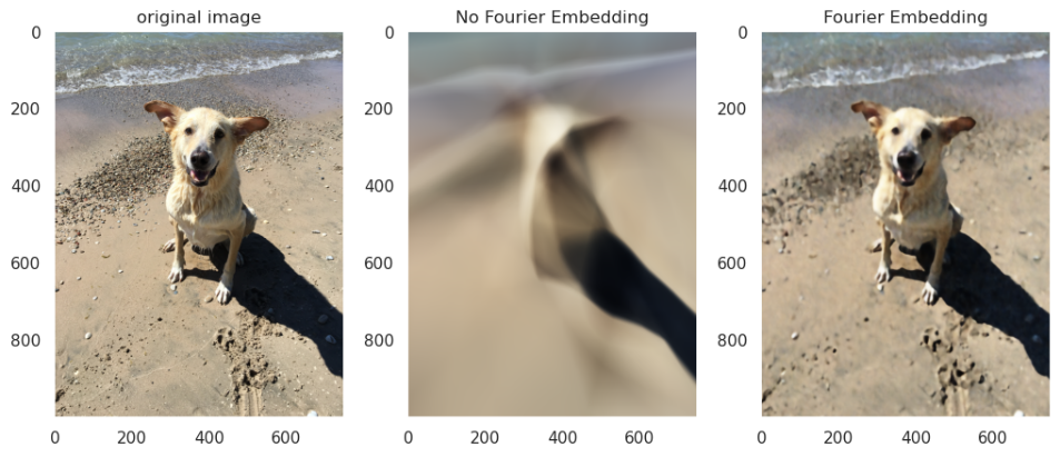
While the Fourier network does not capture every detail, it is able to capture significantly more details than the naive feedforward net.
An aside on nets and compression
The above example can be seen as evidence that deep learning is a kind of lossy, continuous compression. This idea has been popularized by Ted Chiang in the context of GPT, and the relationship between compression and deep learning is quite explicit in the case of Fourier feature networks.
In particular, both the naive feedforward network and the Fourier network constructed above are “compressed” representations of the original image. The image has 1000 $\times$ 700 $\times$ 3 = 2,100,000 free parameters defining it. Our Fourier network has 2 $\times$ 31 + (64 + 1) $\times$ 256 + 2 $\times$ ( (256 + 1) $\times$ 256) + ((256 + 1) $\times$ 3) = 149,057 parameters. And 149,057 < 2,100,000, so we have indeed “compressed” some information. (Observe that the use of trigonometric functions in the compression is, at least at a very high level, similar to the use of the discrete cosine transform in JPEG compression.)
The compression method is also very interesting: the image itself is essentially a discrete function which is only defined at certain points; explicitly it is only defined on the integer lattice $\left[0, 700\right] \times \left[0, 1000\right]$. In contrast, our Fourier network is defined across all of $\mathbb{R}^2$; enter an input like $(x,y)$ = (501.25, 70.341) and it will dutifully produce an output (even though no such point existed in the training set or the original image).
The argument that folks like Ted Chiang are making is that “compression as a continuous function” is a general analogy for what neural nets are doing, applicable beyond just this image reconstruction case. Although this is sometimes proposed as an antidote to the anthropomorphic interpretation of LLMs, I would argue that these are actually complimentary viewpoints: compression is understanding, in the sense that a perfect model precisely describes the mathematical/statistical relationship between its covariates, up to whatever intrinsic noise exists in the problem.
Using Fourier features for portfolio construction
The ability to create smooth, continuous approximations to low-dimensional functions (with a configurable “granularity” parameter—the scale of the Gaussian noise), on its own, is interesting but perhaps not a new capability. For example, smoothing splines are commonly used for both visualization of time series data, and sometimes for various modeling tasks (such as approximating the volatility surface). However, unlike splines, Fourier feature networks are neural networks—and therefore both differentiable and easy to integrate into other network architectures. Let’s take a look at a specific example: implicit factor modeling. First, a quick reminder.
What are implicit factor models?
The idea behind a factor model is that the performance of some group of instruments (say, stocks) is determined by their exposure to various factors. Mathematically, this looks like:
\[\delta_{n} = \alpha_{n} + \sum_{k} \beta_{n,k} f_{k} + \varepsilon_{n}\]where $\delta_{n}$ is the return of instrument $n$, $f_{k}$ are the “factors”, $\beta_{n,k}$ is the exposure of the instrument to that factor (its loading), $\alpha_{n}$ is the performance not explained by the factors, and $\varepsilon_{n}$ is noise.
Across a family of instruments, this looks like:
\[\underbrace{\left[\begin{matrix}\delta_{1}\\ \delta_{2}\\ \vdots\\ \delta_{N} \end{matrix}\right]}_{:=\Delta}=\underbrace{\left[\begin{matrix}\alpha_{1} & \beta_{1,1} & \cdots & \beta_{1,K}\\ \alpha_{2} & \beta_{2,1} & \cdots & \beta_{2,K}\\ \vdots\\ \alpha_{N} & \beta_{N,1} & \cdots & \beta_{N,K} \end{matrix}\right]}_{:=B}\underbrace{\left[\begin{matrix}1\\ f_{1}\\ \vdots\\ f_{K} \end{matrix}\right]}_{:=F}+\varepsilon\]Assuming that the noise terms $\varepsilon_{n}$ are uncorrelated across instruments, then the symbol covariance matrix $\Sigma_{\Delta}$ can be expressed from the factor covariance matrix $\Sigma_{F}$ as:
\[\Sigma_{\Delta}=B\Sigma_{F}B^{T}+D\]where $D$ is the diagonal matrix $D_{ij} = Var(\varepsilon_{n})$.
The key observation is that, when the number of symbols $N$ is much larger than the number of factors $K$, this is a kind of dimensional reduction: there are fewer free parameters on the right-hand side of the equation above than on the left. (In particular, there are $N \times (N - 1) / 2$ parameters on the left, but only $N \times K + K \times (K - 1) / 2 + N$ parameters on the right.)
Simulating some data
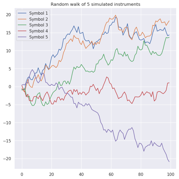
Now suppose we have picked our favorite instruments. For exploratory purposes, let’s create five symbols with a nontrivial covariance matrix:
\[\Sigma=\left[\begin{matrix}1.0 & 0.66 & 0.40 & -0.28 & -0.17\\ 0.66 & 1.0 & 0.26 & 0.43 & -0.61\\ 0.40 & 0.26 & 1.0 & 0.10 & -0.64\\ -0.28 & 0.43 & 0.10 & 1.0 & -0.53\\ -0.17 & -0.61 & -0.64 & -0.53 & 1.0 \end{matrix}\right]\]Simulating random walks of these symbols for 100 steps yields a plot like this:
Let’s try to fit a two-factor implicit factor model on these symbols. For simplicity we will assume that $\alpha_n = 0$ (our symbols have mean zero return), and that $E(f_{k}) = 0$ (i.e., that our factors also have mean zero). Since this will eventually (I promise!) connect back to Fourier features, let’s do this in PyTorch:
class FactorModel(nn.Module):

    def __init__(self, n_symbols: int = 5, n_factors: int = 2):
        super().__init__()
        self.n_symbols = n_symbols
        self.n_factors = n_factors
        # `f_arr` determines the factor covariance matrix
        self.f_arr = nn.Parameter(
            torch.randn((self.n_factors, self.n_factors))
        )
        self.loadings = nn.Parameter(
            torch.randn((self.n_symbols, self.n_factors))
        )
        self.symbol_noise = nn.Parameter(
            torch.randn(self.n_symbols)
        )

    @property
    def factor_cov(self):
        # We need this to be positive semidefinite
        return self.f_arr.transpose(1,0) @ self.f_arr

    @property
    def cov(self):
        return (
            self.loadings
            @ self.factor_cov
            @ self.loadings.transpose(1, 0)
            + torch.diag(self.symbol_noise**2)
        )

    def forward(self, X):
        # Forward pass computes the log probabilities
        # of the observed data, given the factor model
        # assumption
        d = (
            dists
            .multivariate_normal
            .MultivariateNormal(
                torch.zeros(self.n_symbols),
                self.cov
            )
        )
        return d.log_prob(X)
The training loop for this kind of model is very easy—the optimization criterion is just the negative log likelihood of the input sequence:
optimizer = optim.Adam(model.parameters())
for _ in range(N_EPOCHS):
    optimizer.zero_grad()
    yhat = model(obs)
    loss = -1 * yhat.mean() # negative log likelihood
    loss.backward()
    optimizer.step()
After training, here’s the predicted instrument covariance matrix:
\[\hat{\Sigma_{\Delta}}=\left[\begin{matrix}1.0 & 0.09 & 0.12 & 0.07 & -0.16\\ 0.09 & 0.97 & 0.33 & 0.21 & -0.47\\ 0.12 & 0.33 & 0.91 & 0.27 & -0.59\\ 0.07 & 0.21 & 0.27 & 0.79 & -0.38\\ -0.16 & -0.47 & -0.59 & -0.38 & 0.84 \end{matrix}\right]\]and for completeness, the loadings and factor covariances:
\[B,\Sigma_{F}=\left[\begin{matrix}0.58 & -0.75\\ 0.62 & -0.52\\ 0.49 & -1.50\\ 0.17 & -0.10\\ -0.51 & 1.03 \end{matrix}\right],\left[\begin{matrix}4.62 & 1.75\\ 1.75 & 1.07 \end{matrix}\right]\]Fourier factor models
Factor models are a widely used in quantitative finance. However, the technique described above is limited: factors are assumed to be static over the modeling interval. That is, a factor model will struggle to model situations in which the correlation structure between instruments changes over time.
Let’s introduce exactly that situation into our simulated data. Below, I have combined samples from two different multivariate Gaussian distributions to create simulated instruments. In particular, prior to $t = 100$, the correlation matrix is the same as above, whereas afterwards, symbol correlations are completely different.
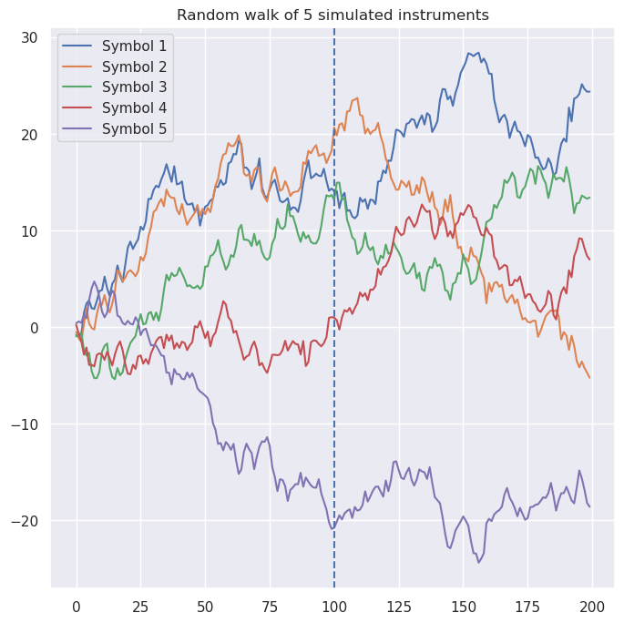
For example, note that symbols 1 and 2 were positively correlated (covariance = 0.62) prior to the shift, and are now weakly negatively correlated (-0.33).
Incorporating this temporal dependence into our factor model is fairly straightforward.
The primary change is the introduction of a new argument, t, representing the temporal dependence of the model.
t = torch.linspace(0, 1, steps=200).unsqueeze(1)
The updated factor model is below, with comments indicating the main changes inline.
class FourierFactorModel(nn.Module):

    def __init__(self, n_symbols: int = 5, n_factors: int = 2):
        super().__init__()
        self.n_symbols = n_symbols
        self.n_factors = n_factors
        # The factor array now has a temporal dependence.
        # The FourierEncoding layer allows us to control
        # the sensitivity of the model to the time variable:
        # increasing the scale or the dimension of the output
        # layer increases the model's ability to discriminate
        # between different points in time.
        self.f_arr = nn.Sequential(
            FourierEncoding(1, 15, scale=1),
            nn.Linear(15, n_factors*n_factors)
        )
        self.loadings = nn.Parameter(
            torch.randn((self.n_symbols, self.n_factors))
        )

        self.symbol_noise = nn.Parameter(
            torch.randn(self.n_symbols)
        )

    def factor_cov(self, t):
        f_mat = (
            self
            .f_arr(t)
            .reshape(-1, self.n_factors, self.n_factors)
        )
        # The first index is the batch index, and we
        # want to do matrix multiplication along the
        # latter two indices.
        return f_mat.transpose(2, 1) @ f_mat

    def cov(self, t):
        return (
            self.loadings
            @ self.factor_cov(t)
            @ self.loadings.transpose(1, 0)
            # Note the unsqueeze; the assumption here is
            # that the residual noise is identically distributed
            # in time.
            + torch.diag(self.symbol_noise**2).unsqueeze(0)
        )

    def forward(self, t, X):
        d = (
            dists
            .multivariate_normal
            .MultivariateNormal(
                # Note that the center of the distribution
                # must again be shape (batch_size, n_symbols)
                torch.zeros((t.shape[0], self.n_symbols)),
                self.cov(t)
            )
        )
        return d.log_prob(X)
The training loop is much the same as it was before:
model = FourierFactorModel(5, 2)
t = torch.linspace(0, 1, steps=200).unsqueeze(1)
optimizer = optim.Adam(model.parameters())

for _ in range(N_EPOCHS):
    optimizer.zero_grad()
    yhat = model(t, obs_full)
    loss = -1 * yhat.mean()
    loss.backward()
    optimizer.step()
And, at least on this small generated dataset, yields a nice loss curve:
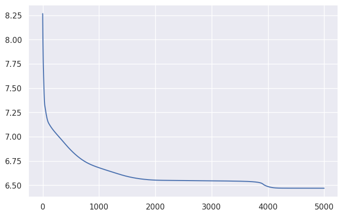
Of course, the real question is, does this model capture the changing correlations between our simulated instruments?
To answer that question, let’s first spot-check a few pairs. One of the biggest swings was the relationship between Symbol 1 and Symbol 2: prior to $t = 100$, $Cov(S1, S2) = 0.66$, whereas afterward, $Cov(S1, S2) = -0.32$. Two other notable changes were between Symbol 3 and Symbol 5 ($-0.64$ to $0.17$), and between Symbol 4 and Symbol 5 ($-0.53$ to $0.52$). And here are the predicted covariances from our factor model, for these symbols:
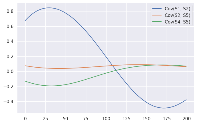
To my eye, it looks like the model largely captured the changing relationship between Symbol 1 and 2, but missed the other two changes. There are a few reasons why this might be the case. For one thing, there’s an element of randomness to this entire exercise: by plotting the true log probabilities of our sequences, we can see that the steps prior to $t=100$ were generally closer to the expected value than those afterwards.
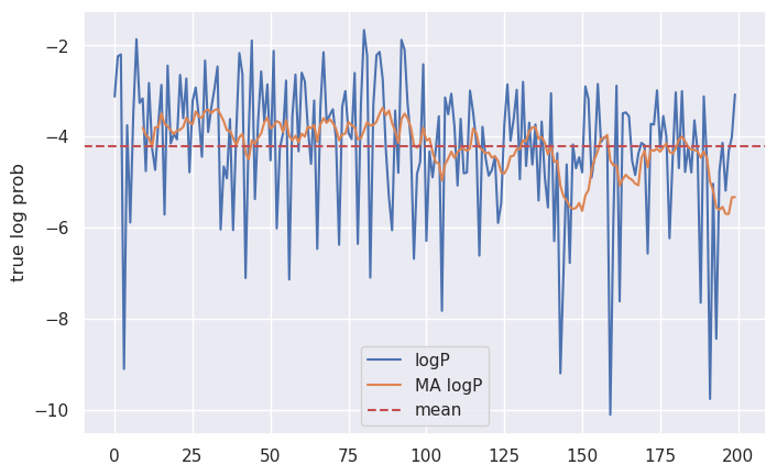
This suggests that we should anticipate more error in the model’s predictions toward the latter half of the sequence than at the beginning.
Note also that there’s an element of randomness to the initialization of this model: depending on the random seed, it will construct wildly different implicit factors. This might be addressed by, for example, initializing the loadings and initial factor array such that they best match the empirical covariance matrix, or treating the temporal dependence as a perturbation of the “time-constant” factor model. We might also “freeze” the loading matrix $B$ to that produced by more traditional methods (e.g. PCA).
All of this is somewhat beyond the scope of this blog post, however—the main point I want to illustrate is that using Fourier-encoded features on low-dimensional data allows us to use nets to model low-dimensional phenomena. Images (a two-dimensional input) were one example of this, but this approach to implicit factor modeling shows that the technique is not limited to computer vision.