Everything I know about Deep Learning (II)
What is deep learning? How does it work? Why does it work? This is part 2 of a 3 part series on deep learning. In this post we’ll focus on the how: how does deep learning work? You can find part 1 here and part 3 here.
How does deep learning work?
Recall from last time that (dense, feed-forward) neural nets are just stacked linear models:
\[\hat{y}=W_{3}\left(\sigma\left(W_{2}\left(\sigma\left(W_{1}x+b_{1}\right)\right)+b_{2}\right)\right)+b_{3}\]In a literal sense, this equation is all you need to explain “how” a neural net works:
- An input vector $x$ is passed through an affine transformation
- Then, a nonlinear “activation” function is applied elementwise to the result
- This is repeated until the output $\hat{y}$ is produced.
While the above is true, it’s an unsatisfying explanation. Fortunately, we can go a little deeper, in two ways:
- Does the mathematical structure described above provide any intuition about a net’s outputs in general?
- In practice, how do we actually find the net’s parameters $W_i$ and $b_i$?
Let’s start first with the practical side of this question: how do we discover the net’s parameters?
How do you train a neural net?
In the previous post, we framed building a neural net as a type of optimization problem. Here’s a brief recap:
- A net can be thought of as a parameterized function $f_{\theta} : \mathbb{R}^n \rightarrow \mathbb{R}^m$, where $\theta$ is some vector specifying the elements of the matrices $W_i$ and vectors $b_i$. (That is, $\theta \in \mathbb{R}^K$, where $K$ is the number of free parameters of the network—and often $K$ is very large.)
- For a set of training data \(X, Y = \{(x_i, y_i)\}_{i=1}^{N}\), we want to choose $\theta$ such that $f_{\theta}(x_i) \approx y_i$
- To make this notion of “approximately equal” precise, we have to introduce a loss function $\mathcal{L}_{X,Y}(\theta)$ and choose $\theta$ to minimize this loss function
We also introduced two common choices of loss function. They are the mean squared error:
\[\mathcal{L}_{X,Y}^{MSE}(\theta) = \frac{1}{N} \sum_{i=1}^{N} (y_i - f_{\theta}(x_i))^2\]which we motivated as the optimization criterion that maximizes the log of the likelihood function under the assumption that the model’s errors are Gaussian. And, for categorical problems, we introduced the categorical cross entropy:
\[\mathcal{L}_{X,Y}^{CE}(\theta) = \sum_{i=1}^{N} \sum_{l} 𝟙_{y_i = l} \log (P_{\theta} (y = l | x_i))\]where $l$ are the set of possible output labels, \(P_{\theta}(y = l | x_i)\) are the probabilities predicted by the model $f_\theta$ and \(𝟙_{y_i = l}\) the indicator function (1 if $y_i = l$, 0 otherwise). (As a practical matter, note that it is often better to have your model produce log probabilities: usually a softmax function is applied to the model’s outputs to ensure that all probabilities add up to 1, and taking the log of this can introduce numerical instabilities.)
Now that we’ve framed this as an optimization problem (find $\theta$ that minimizes \(\mathcal{L}(\theta)\)), we have to actually solve the optimization problem. Numerical optimization is a broad subject, and there are a lot of possible ways to solve this optimization problem. However, recall that $\theta \in \mathbb{R}^K$ for some often very large $K$—many optimization algorithms (e.g. simulated annealing) do not scale well to high dimensions. In a very high-dimensional space, there’s really only one sensible choice, and that’s gradient descent.
Gradient descent
The gradient of a function $f(x_1, x_2, \ldots, x_n)$ is a vector $\nabla f$ defined by
\[\nabla f = \frac{\partial f}{\partial x_1} \hat{x_1} + \frac{\partial f}{\partial x_2} \hat{x_2} + \cdots + \frac{\partial f}{\partial x_n} \hat{x_n}\]As we showed last time, the gradient of the function actually defines a vector field on the function’s domain, and this vector field is perpendicular to the level sets of the function at every point. Moreover, for convex functions the flow of this vector field (the gradient flow line) will define a curve that originates at the function’s minimum and terminates at its maximum. We can approximate this gradient flow line (and hence numerically minimize our function) by iteratively taking small steps in the direction defined by the gradient vector field—this is the gradient descent algorithm.
In contrast to many other optimization techniques, gradient descent’s complexity scales linearly with the number of dimensions: only one additional gradient term needs to be calculated if $\theta \in \mathbb{R}^{K + 1}$ as opposed to $\theta \in \mathbb{R}^{K}$. Contrast this with a technique like Newton’s method, which will theoretically take a shorter path to the optimum than gradient descent, but requires calculating the Hessian, a calculation that grows $\mathcal{O}(n^2)$ with increasing dimension.
To actually use gradient descent for our problem, however, we need an efficient way to compute the terms in $\nabla \mathcal{L}(\theta)$. (If you’re not interested in how gradients are calculated under the hood, you may safely skip ahead to the next section.) Enter automatic differentiation.
Automatic differentiation
Our neural net looks something like:
\[\hat{y}=W_{3}\left(\sigma\left(W_{2}\left(\sigma\left(W_{1}x+b_{1}\right)\right)+b_{2}\right)\right)+b_{3}\]that is, it is a chain of compositions of affine transformations and activation functions. In principle we could estimate the gradient vector numerically, for each $\theta_j$, by the definition
\[\nabla_{\theta_j} \mathcal{L}(\theta) = \lim_{h \rightarrow 0} \frac{\mathcal{L}(\theta + h \hat{\theta_j})}{h}\]That is, for each individual parameter, add a small offset $h « 1$, compute $\mathcal{L}$, normalize by $h$, and then combine the results to approximate $\nabla \mathcal{L}(\theta)$. In practice this is a very inefficient and potentially error-prone way to do this calculation: I have to repeat the evaluation of the entire loss function for every single parameter in my net, and the result is only approximately correct.
Moreover, by design, I actually know (as in, can write an analytic expression for) the derivatives of each layer in my network: the elementwise activation function just has derivative \(\dot{\sigma}\), and the affine terms have derivative \(W_{k}\). So, if I carefully track derivatives of each component in my net and use the chain rule, I can get the gradients I need very efficiently. This is the idea behind automatic differentiation.
Here’s how it works:
First, recall the chain rule—if I have a function $y = f(g(h(x)))$, then
\[\frac{dy}{dx} = \frac{dy}{df} \frac{df}{dg} \frac{dg}{dh} \frac{dh}{dx}\]Let’s write
\[w_0 = x\] \[w_1 = h(w_0)\] \[w_2 = g(w_1)\] \[w_3 = f(w_2) = y\]Then the chain rule above becomes
\[\frac{dy}{dx} = \frac{dw_3}{dw_2} \frac{dw_2}{dw_1} \frac{dw_1}{dw_0}\]There are now two recursive relationships between the $w_i$’s:
- \[\frac{dw_i}{dx} = \frac{dw_i}{dw_{i-1}} \frac{d w_{i-1}}{dx}\]
- \[\frac{dy}{dw_i} = \frac{dy}{dw_{i+1}} \frac{dw_{i+1}}{dw_i}\]
This means we can compute the components of the chain rule iteratively, either right to left (“forward accumulation”, using relationship 1) or left to right (“reverse accumulation”, using relationship 2).
Now suppose that I have two functions $f(x) = ax + b$ and $g(x) = sin(x)$, and I want to compute the gradient of the composite function $y = g(f(x))$. Setting $w_0 = x$, $w_1 = f(w_0)$, $w_2 = g(w_1) = y$, I can compute the derivative of $y$ in two ways. First, via forward accumulation:
- $w_0 = x$ implies $\frac{dw_0}{dx} = 1$.
- $w_1 = aw_0 + b$, so
- and $w_2 = \sin(w_1)$, so
For reverse accumulation, we go the other way around:
- \[\frac{dy}{dw_2} = 1\]
- \[\frac{dy}{dw_1} = \frac{dy}{dw_2} \frac{dw_2}{dw_1} = 1 \cdot \cos(w_1)\]
- \[\frac{dy}{dw_0} = \frac{dy}{dw_1} \frac{dw_1}{dw_0} = (1 \cdot \cos(w_1)) \cdot (a)\]
- \[= a \cos(ax + b)\]
We’ve now calculated the derivative $\dot{y}$ using the chain rule in two different ways. And, as a practical matter, if I keep track of the values of the partial derivatives of each component function, then whenever I evaluate $y = g(f(x))$ for some specific input $x_0$, I also get the derivative \(\left.\frac{dy}{dx}\right|_{x=x_0}\) at $x_0$ for only a little extra computational overhead.
But so what?
The point is this: if we have some general function formed from a composition of primitives, where we know the derivative of each primitive, we can actually compute the gradient of that general function at any input, just by tracking a small piece of additional information (the $\dot{w_i}$’s).
In fact this is exactly what automatic differentiation libraries like Flux, PyTorch, and JAX are doing.
Backpropagation
This turns out to also be the crucial tool we need to efficiently compute gradients for our neural nets. Consider our loss function \(\mathcal{L}_{X,Y}(\theta)\). All of the loss functions we’ve seen so far actually look something like this:
\[\mathcal{L}_{X,Y}(\theta) = ``\int_{X}" L(y, f_{\theta}(x))\]where “integrate” in this case means some kind of sum over the training set (e.g. a mean). Let’s use \(\frac{d\mathcal{L}}{d \theta}\) to represent the total derivative of the loss function. (Note that this total derivative is just the transpose of the gradient vector, or, if you’re a math PhD and feeling fancy, it’s the differential 1-form given by the exterior derivative of $\mathcal{L}$.) Using the Leibniz rule, we may safely commute “integration” with differentiation, so let’s just zoom in on \(\frac{d L}{d \theta}\).
For a generic dense feedforward neural net with $K$ layers, we have:
\[f_{\theta}(x) = \sigma \left( W_{K} \left( \sigma \left( W_{K-1} \left( \cdots W_1 x + b_1 \right) \right) \right) \right)\]For simplicity, let’s assume that all the $b_j = 0$ (any affine transformation from \(\mathbb{R}^n \rightarrow \mathbb{R}^m\) looks like the composition of a linear transformation \(W : \mathbb{R}^{n+1} \rightarrow \mathbb{R}^m\) with the projection $\pi (x_1, x_2, \ldots, x_{n+1}) = (x_1, x_2, \ldots, x_n, 1)$, so we can make this assumption without loss of generality.) Then, using the $w_i$ automatic differentiation notation for each stage in the composition, and \(\tilde{w_i} := \sigma (w_i)\) , we have
\[\frac{dL}{dx} = \frac{dL}{d \tilde{w_K}} \frac{d \tilde{w_K}}{d w_K} \frac{d w_K}{d \tilde{w_{K-1}}} \cdots \frac{d w_1}{d x}\]The derivatives of the activation function are the same everywhere (just the diagonal matrix whose nonzero entries are all $\dot{\sigma}$, which I will also refer to as $\dot{\sigma}$). And the terms $\frac{d w_j}{d \tilde{w_{j-1}}}$ are the derivatives of the affine transformation $x \mapsto W_j x$. Putting this together, we have
\[\frac{dL}{dx} = \frac{dL}{d \tilde{w_K}} \dot{\sigma} W_K \dot{\sigma} W_{k-1} \cdots W_{1}\]To get the gradient, we need only take the transpose:
\[\nabla_{x} L = W_1^T \cdot \dot{\sigma} \cdots W_{K-1}^T \cdot \dot{\sigma} W_{K}^T \cdot \dot{\sigma} \cdot \nabla_{\tilde{w_K}} L\]Now, we may apply reverse accumulation to this quantity to discover the derivatives with respect to each component:
\[\frac{dL}{d w_i} = \frac{dL}{d w_{i+1}} \frac{d w_{i+1}}{d w_i}\]This yields
\[\nabla_{W_j} L = \dot{\sigma} \cdot W_{j+1}^T \cdots \dot{\sigma} W_{K-1}^{T} \cdot \dot{\sigma} W_{K}^T \cdot \dot{\sigma} \nabla_{\tilde{w_K}} L\]and starting at the outermost layer $W_K$, we can recursively compute each of the derivatives we need.
The reason this is called “backpropagation” is that the “errors” of the net ($\nabla_\tilde{w_K} L$) are propagated backwards (from the outermost layer inward) during the gradient computation. It’s important to note, however, that backpropagation is just an efficient way of calculating gradients (and a specific application of automatic differentiation)—the end result is still the gradient.
Interpreting a net’s outputs
Now that we understand automatic differentiation, let’s take stock of where we’re at.
- We can write out our net $f_\theta$ as an explicit chain of affine transformations and nonlinear activation functions, parameterized by some vector $\theta$
- We have some loss function \(\mathcal{L}_{X,Y}(\theta)\) which describes the performance of our net $f_\theta$ on a training set $X, Y = {(x_i, y_i)}$
- We can efficiently compute the gradients $\nabla_{\theta} \mathcal{L}$ using automatic differentiation
- Using the above, we can try to find the optimal $\theta$ via gradient descent
What does this tell us about how a net actually works? There are a number of perspectives we can take on how to interpret what a neural net is doing when it makes a prediction, and “interpretable machine learning” is an active area of research. Rather than try to give a rushed account of the literature, I will instead focus in on two perspectives that have been most useful to me.
Perspective 1: Latent representations
Last time we talked briefly about a net’s latent spaces. For example, for the following net
\[\hat{y}=W_{3}\left(\sigma\left(W_{2}\left(\sigma\left(W_{1}x+b_{1}\right)\right)+b_{2}\right)\right)+b_{3}\]the variable $\tilde{x}$ defined by
\[\tilde{x} := \sigma\left(W_{2}\left(\sigma\left(W_{1}x+b_{1}\right)\right)+b_{2}\right)\]is a “latent representation” of the input $x$ produced by partially applying the network. The space of all such $\tilde{x}$ is a latent space of the network, and it is geometrically interesting:
On the final latent space, the net reduces to a linear model:
\[\hat{y} = W_3 \tilde{x} + b_3\]Because of this, our intuitions about linear models transfer to the net’s actions on the latent space. An important fact about affine maps (such as the above net’s action on this latent space) is that they preserve linear structure on the domain, e.g., if three inputs \(\tilde{x}_1\) , \(\tilde{x}_2\) , \(\tilde{x}_3\) are colinear, then their outputs \(\hat{y}_1\) , \(\hat{y}_2\) , \(\hat{y}_3\) will also be colinear. Note that affine maps are not necessarily conformal, e.g., if the \(\tilde{x}_i\) ‘s form a right triangle in the latent space, the output triangle formed by the \(\hat{y}_i\) ‘s may not have the same angles—so we cannot draw too much intuition about the directions in the latent space. Nevertheless, the affine nature of this map lets us infer some useful properties.
Let’s consider a concrete example.
An example: bond trading
Suppose we are bond traders, and we want to build a “bond comparison” tool that, for a given bond, lets us find other bonds that are similar to it. We can attack this problem using the latent representation produced by a net.
As far as financial instruments go, bonds are a little tricky in that they trade infrequently and they are also not very fungible: a $1000 bond with a 1% coupon that matures in 12 months from company XYZ may trade differently than one with the exact same principal, coupon, and maturity characteristics from company ABC. Moreover we have lots of potentially interesting information about a given bond that we can include in our model: the creditworthiness of the issuer and other features about the company, the origination date, the coupon frequency, etc, and we may not know which features are relevant.
We are bond traders, so we are interested in ranking bonds by similarity with respect to trading, i.e., bonds that should be priced similarly. Ordinarily a reasonable first guess for what the next price that something will trade at is whatever price it last traded at. But, because many bonds trade infrequently, this pricing information is often stale—sorting bonds by last trade might not be good enough for us. (Plus, this is a blog post about neural nets, so we’ve gotta use nets somewhere.)
Suppose we train a neural net to estimate the next trade price for a bond, using whatever features of the bond we think might be informative. In addition to the estimated price \(\hat{y}\), for each bond $x$, we also have a latent representation \(\tilde{x}\) . This latent representation can be thought of as providing some number of “derived” features that are most predictive of the next trading price of the bond. We control how many of these derived features there are (by controlling the dimension of the latent space). The larger the size of the latent space, the sparser the representation will be, so if we want a dense embedding of our inputs, we should pick a low dimension. (By “dense embedding”, I mean an embedding which is not “sparse”: if we collect all of the vector representations of our observations and arrange them into the columns of a matrix, the embedding that generated those representations is sparse if there’s some change of basis such that that matrix is mostly zeroes; intuitively this means that most dimensions of our embedding are not shared across observations. The classic example of a sparse embedding is one-hot encoding—each observation $x_i$ gets mapped to a vector which is entirely zeroes, except for a 1 in the $i$th entry.)
And now we have constructed a powerful tool: Bonds whose latent representations are close are bonds who our model expects to trade similarly. So, to build our bond comparison tool, for a given bond, all we need to do is rank other bonds by their latent space distance to the point of comparison.
Word vectors
Clever use of latent space representations turns out to be the same idea behind constructing word vectors, most classically via Word2Vec.
In Word2Vec and related approaches, the model is trained to predict the next token (or set of tokens) in a sequence. The simplest version of this approach looks something like this:
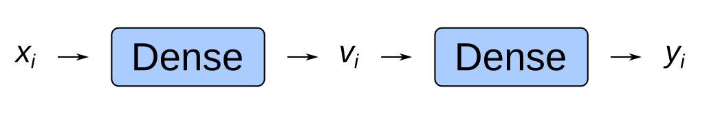
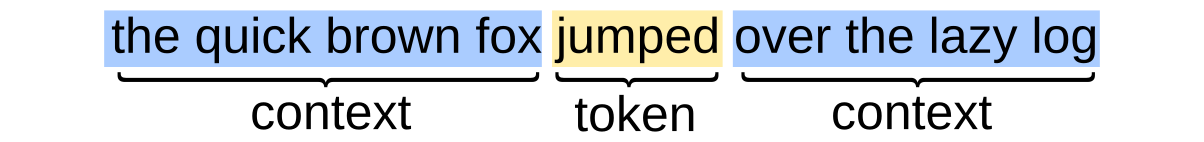
Each input $x_i$ is a “bag of words” representation of the context for the token, that is, a vector whose $k$th entry indicates whether or not the $k$th word from the corpus is present in the context.
For example, if my vocabulary consists of the three tokens “A”, “B”, and “C”, then the sentence "A C" would be encoded as (1, 0, 1) (and so would the sentences "A A C", "C A C", etc).
The output is a list of class probabilities for the token in the sequence. The predictions of the model are actually not that interesting—instead, the item of interest is the interior latent representation $v_i$, which is a dense vector (classically of dimension 100, though more recent approaches use larger representations).
Applying the same affine algebra to the latent space (that is, the “word vectors” produced by this model) yields some interesting results. Words that are synonyms often have very similar vector representations. Additionally, you can do arithmetic on word vectors, for example:
\[\mathtt{king}-\mathtt{man} \approx \mathtt{queen}-\mathtt{woman}\]which seems to capture something like analogy relationships. (The $\approx$ in the equation above means that the points in latent space on the left-hand-side and right-hand-side above are very close.)
This kind of result can be seen as evidence in favor of the distributional hypothesis (which claims that words with similar statistical properties have similar meanings), in that the word representations learned by the model entirely from co-occurrence frequencies seem to capture some semantic information about the word itself. But that’s a bit of a digression! Much has been written about word vectors, and if you’re interested in this kind of thing, there’s a fun introduction here.
Now let’s take a look at the second perspective.
Perspective 2: Nets are approximately piecewise linear
Let’s return once again to our formula for a dense, fully connected network with 3 hidden layers:
\[\hat{y}=W_{3}\left(\sigma\left(W_{2}\left(\sigma\left(W_{1}x+b_{1}\right)\right)+b_{2}\right)\right)+b_{3}\]Historically, the activation function $\sigma$ was the “sigmoid” function
\[\sigma(x) = \frac{e^{x}}{e^{x} + 1}\]This function has an annoyance in practice, however: its derivative is
\[\frac{d \sigma}{dx} = \frac{e^{x}}{\left(1 + e^x \right)^2}\]and this derivative rapidly vanishes as $x \rightarrow \pm \infty$ , as shown below:
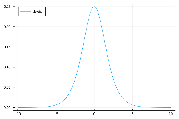
As we now know from the previous section on automatic differentiation, the gradient of our net will include multiples of the activation function’s derivative—meaning that, for a net with many hidden layers, we may see vanishing gradients.
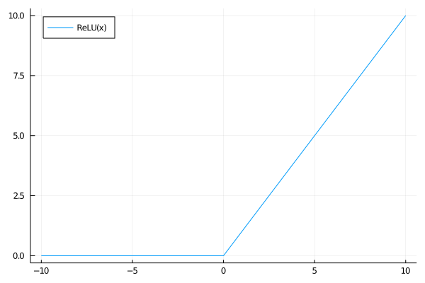
To remedy this, more recent nets use different activation functions. The most popular is the “rectified linear unit” (ReLU) function, defined by
\[\text{relu}(x)=\begin{cases} x & x\geq0\\ 0 & x<0 \end{cases}\]This function has the property that its derivative is the step function (0 when $x < 0$, 1 when $x > 0$ ), so we avoid the vanishing gradient problem.
Let’s suppose that we use a ReLU activation instead of a sigmoid one. What does this tell us about our network?
ReLU is a piecewise linear function: for any \(x \in \mathbb{R}\), there exists some $x_0 \leq x$ and $x_1 \geq x$ such that, on the domain $[x_0, x_1]$, \(\sigma(x) = a x + b\).
Lemma: If $f$ and $g$ are two piecewise linear functions, then the composition $f(g(x))$ is also piecewise linear.
Proof: Let \(y = g(x)\). Then, by definition, there exist $x_0$ , $x_1$ , $a$ , and $b$ , such that $y = a x + b$ for $x_0 \leq x \leq x_1$ . And there exist $y_0$ , $y_1$, $c$ , and $d$ , such that $f(y) = c y + d$ for $y_0 \leq y \leq y_1$ . Without loss of generality, let’s assume that $a > 0$ and $c > 0$ (we only need this to cleanly express the linearity interval for $x$).
Then, \(f(g(x)) = (ac) x + (bc + d)\) for
\[\max \left(\frac{y_0 - (bc + d)}{ac}, x_0\right) \leq x \leq \min \left(\frac{y_1 - (bc + d)}{ac}, x_1 \right)\]and thus $f(g(x))$ is piecewise linear.
Finally let’s consider a multidimensional function \(f:\mathbb{R}^n \rightarrow \mathbb{R}^m\). Let’s say that such a function is piecewise linear if it is piecewise linear in each of its components, i.e., if $f_j (x_1, x_2, \ldots, x_n)$ is piecewise linear in $x_k$ for all $1 \leq j \leq m$ and $1 \leq k \leq n$ .
Then, neural nets with ReLU activation are piecewise linear!
This can be seen explicitly in a one-dimensional case. Below is the plot of the in-sample and out-of-sample predictions of a neural net with ReLU activation fit to minimize MSE using 10 points randomly sampled from a sine wave:
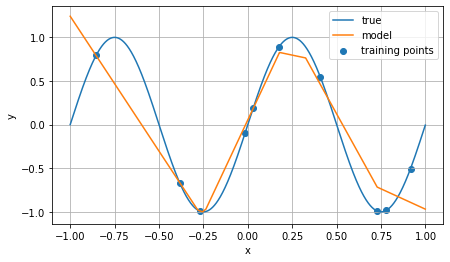
The line in blue is the “ground truth” data; the blue dots are the 10 points used for training, and the line in orange is the net’s predictions on the domain.
Observe that the net is indeed, as claimed, a piecewise linear function. This is actually a pretty powerful property: it tells us that, in order to make a prediction on an input, the net will linearly interpolate between the “hinge points” (the ends of the line segments) chosen by the net during training. I draw two intuitions from this:
First, for a given input, to make a prediction, the net is essentially finding some set of nearby input-output pairs it memorized during training, and then producing a prediction by linearly interpolating between the memorized outputs. This is not precisely correct—for one thing, the hinge points of the piecewise linear function may not correspond to actual input-output pairs seen during training—but it is a rough approximation.
Second, if a new input comes along that is outside of the training domain (in the sine example above, this would be inputs on the left or right side of the graph), the net produces its prediction by linear extrapolation from the values it has already seen. This is one reason why nets outperform other “universal approximators” such as polynomial functions: linear extrapolation is a conservative assumption to make about what happens out of sample (as compared to polynomial extrapolation). Many phenomena look locally linear (that’s basically the core idea of differential geometry), and nets with ReLU activation have that assumption explicitly baked in.
I’ll wrap this post up here. In the final part of this series, we’ll look at areas where nets have been successful (and also some areas where they have not), and I’ll sketch some ideas about why they are so successful.
Special thanks to Eric Z., Honghao G., and Alex S. for their comments on this series!