Everything I know about Deep Learning (I)
Deep learning has achieved widespread use and significant prominence over the past decade, and deep learning models now impact many areas of our lives. But what is deep learning? How does it work? Why does it work? And is it really a path toward general artificial intelligence? I’ll attempt to answer all of these questions and more in this 3-part series.
This post is part 1 of the series. You can find part 2 here, and part 3 here.
What is deep learning?
“Deep learning” is the application of “deep” neural nets to machine learning problems. The “deep” part refers to the use of neural nets with multiple hidden layers. But what is a neural net?
The typical introduction to a neural net begins with a picture like this:
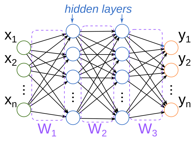
This picture is supposed to be analogous to how biological neural networks work: each circle is a “neuron”, which is connected to subsequent downstream neurons. An incoming signal activates one or more neurons (say, $x_i$), which then propagate activations downstream to other connected neurons, until finally some combination of output neurons (the $y_i$) are activated to produce the response. The “weights” of the network (the $W_j$) determine how activations of upstream neurons influence the activations of downstream ones.
Sounds great, right? There’s only two problems with this story:
- This is not actually how biological neurons work (and we’ve known this for about 50 years now); and
- This isn’t actually how neural nets work in machine learning, either!
To accurately describe how these nets work, it is helpful to start with something smaller. Let’s start with linear regression.
Linear regression
A linear regression is a very simple type of machine learning (really, statistical—although arguably machine learning is a subfield of statistics) model. The problem setup is as follows:
- I have some collection of inputs ${x_1 , x_2, \ldots, x_n}$ where, in the simplest case, $x_i \in \mathbb{R}$ (that is, each $x_i$ is a real number)
- I also have some collection of outputs ${y_1 , y_2, \ldots, y_n}$ where $y_i \in \mathbb{R}$ as well.
From this, I want to construct a function $f:\mathbb{R} \rightarrow \mathbb{R}$ such that $f(x_i) = y_i$, and, importantly, I want $f$ to be affine, i.e., I want $f$ to be of the form
\[f(x) = W x + b\]for some real numbers $W$ and $b$.
In general, unless we’ve been very lucky in our choice of ${x_i}$ and ${y_i}$, such an $f$ will not exist. But, being optimistic folks, we are not deterred by this and will be satisfied if we can find the best possible $f$, that is, the choice of $W$ and $b$ that gets us closest to $y_i$ for each $x_i$.
To be rigorous, I need to tell you what I mean by close—and there are a few choices here. One obvious choice is to minimize the error. Let’s call the quantity $f(x_i) =: \hat{y}i$ . ( $\hat{y}$ is the conventional notation among data scientists for a _predicted value for $y$, whereas the “un-hatted” version indicates the observed value. ) Then the error for an individual prediction is $y_i - \hat{y}_i$ . Note that if $\hat{y}_i » y_i$, then the error is generally large and negative—so minimizing the signed error may not produce predictions that are especially close to the $y_i$. To get around this, we may instead try to minimize the mean absolute error (MAE), that is, choose $W$ and $b$ such that
\[f = \arg \min \frac{1}{N} \sum_{i=1}^{N} \left| y_i - \hat{y}_i \right|\]( \(\arg \min f(x)\) is the “minimizing argument of $f$ “, that is, a value $x$ which minimizes $f$ .)
Maximum likelihood estimation
The choice of mean absolute error may feel a little arbitrary to you. If, like me, you enjoy thinking probabilistically, you could instead assume that the errors of our model follow some probability distribution $\mathcal{D}$, in which case we can write the model as:
\[y - (W x + b) \sim \mathcal{D}\]and then seek to choose $W$ and $b$ to maximize the probability (with respect to our model) of seeing the particular batch of observations ${(x_i, y_i)}$ that we happened to observe:
\[P(y_i | x_i, W, b, \mathcal{D}) = \prod_{i=1}^{N} P_{\mathcal{D}}(y_i - (W x_i + b))\]People like to (often incorrectly!) assume that $\mathcal{D}$ is a normal distribution $\mathcal{N}(0, \sigma)$ with some variance $\sigma ^2$. In this case,
\[P_{\mathcal{D}}(y_i - \hat{y}_i) = \frac{1}{\sigma \sqrt{2 \pi}} e^{ - \frac{1}{2} \left( \frac{y_i - \hat{y}_i}{\sigma}\right)^2}\]and, taking the logarithm of the previous expression (log is a monotonically increasing function, so this transformation doesn’t affect the optimal arguments), we have
\[\log P(y_i | x_i, W, b) = \sum_{i=1}^{N} -\log( \sigma \sqrt{2 \pi}) - \frac{1}{2} \left( \frac{y_i - \hat{y}_i}{\sigma} \right)^2\]This quantity is called the log likelihood, and we want to find $W$ and $b$ that maximize it, which is equivalent to minimizing $-1 \times \log P$. The resulting optimization criterion (that is, the function we want to minimize) is
\[\mathcal{L}(W, b) = \frac{N}{2} \log(2 \pi) + N \log \sigma + \frac{1}{2 \sigma^2} \sum_{i=1}^{N} \left(y_i - \hat{y}_i \right)^2,\]and if we don’t care about $\sigma$ (or we hold it fixed), the minimal argument to $\mathcal{L}$ will be the same as minimizing the mean squared error (MSE):
\[\mathcal{L}_{MSE}(W, b) = \frac{1}{N} \sum_{i=1}^{N} \left(y_i - \hat{y}_i \right)^2\]So, depending on the assumptions you’re making about the problem (specifically, that errors are normally distributed), the MSE is another very reasonable choice to make for optimization criterion (which I’ll also refer to as a loss function).
In any event, we now have some optimization criterion (MSE, MAE, maybe something else), and we want to find $W$ and $b$. How might we do this?
Assuming that the loss function $\mathcal{L}$ is differentiable with respect to $W$ and $b$, then we could try using gradient descent.
Gradient descent
Recall that the gradient of $\mathcal{L}$ is just the vector of its partial derivatives:
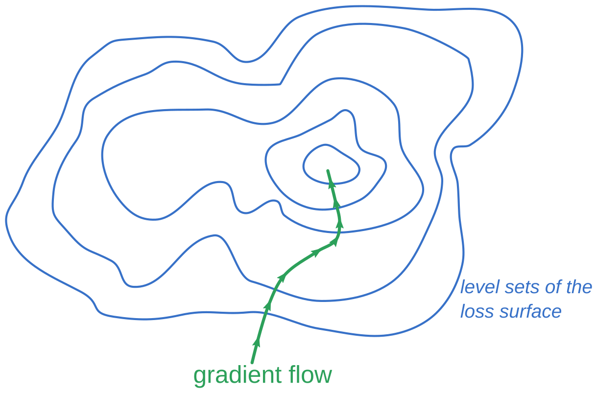
\[\nabla \mathcal{L} = \left( \frac{\partial \mathcal{L}}{\partial W}, \frac{\partial \mathcal{L}}{\partial b} \right)\]Gradients and level sets
It turns out that the gradient vector is always perpendicular to the level sets of the function. In fact, there’s a slick proof:
Let $f:\mathbb{R}^n \rightarrow \mathbb{R}$ be any function. Let $S := f^{-1}(c)$ be a level set. Suppose that $\gamma (t)$ is a curve lying on the level set, with $\gamma(t_0) = p$ for some $p \in f^{-1}(c)$. Then:
\[f(\gamma(t)) = 0\] \[\implies \frac{d}{dt} f(\gamma(t)) = 0\]Applying the chain rule, this is:
\[\frac{\partial f}{\partial x_1} \frac{d x_1}{d t} + \frac{\partial f}{\partial x_2} \frac{d x_2}{d t} + \cdots + \frac{\partial f}{\partial x_n} \frac{d x_n}{d t} = 0\]The left-hand side of this equation is exactly the dot product between the gradient of $f$ and the tangent vector to $\gamma(t)$:
\[\nabla f \cdot \dot{\gamma}(t) = 0,\]so the gradient is perpendicular to the level set at $p = \gamma(t_0)$, which was an arbitrary point on the level set.
Thus, intuitively, the gradient direction is the direction of greatest change in the value of $f$: it is always perpendicular to any “directions of no change” (that is, tangents to the level set).
The gradient defines a vector field on the domain of $f$, so for any point $p_0 \in \mathbb{R}^n$ there’s a curve $\gamma (t)$ defined by
\[\gamma(0) = p_0\] \[\dot{\gamma}(t) = \left. \nabla f \right|_{p = \gamma(t)}\]called the gradient flow line.
When $f$ is a convex function, it can be shown (though I won’t do so here!) that
\[\lim_{t \rightarrow -\infty} \gamma(t) = \arg \min (f)\]That is, if you follow the gradient flow line backward, it will lead you to the minimum.
Numerically approximating the gradient flow
Now let’s return to linear regression. For convenience, let’s bundle our model’s parameters $W, b$ into a vector:
\[\theta := (W, b) \in \mathbb{R}^2\]Any of the loss functions we considered in the previous section can be thought of as functions $\mathcal{L}:\mathbb{R}^2 \rightarrow \mathbb{R}$, so if we choose some initial $\theta^{0} \in \mathbb{R}^2$ and compute the gradient flow line through $\theta^{0}$, we can follow the gradient flow back to the optimal choice of $\theta$. In practice, the gradient flow often does not have an analytic solution (i.e., we can’t just write it out).
However! We can numerically approximate this negative gradient flow by choosing some step size $\alpha \in (0, \infty)$ and iteratively applying the update rule:
\[\theta^{t+1} \leftarrow \theta^{t} - \alpha \nabla _\theta f\]Explicitly, to find the optimal $W$ and $b$, start by picking some random choice $W = W^0$, $b = b^0$. Then, compute the gradient:
\[\nabla\mathcal{L}|_{W^{0},b^{0}}=\left(\left.\frac{\partial\mathcal{L}}{\partial W}\right|_{W=W^{0}, b=b^0},\left.\frac{\partial\mathcal{L}}{\partial b}\right|_{W=W^0, b=b^{0}}\right)\]and loop until the result converges:
\[W^{1}=W^{0}-\alpha\left.\frac{\partial\mathcal{L}}{\partial W}\right|_{W=W^{0},b=b^{0}}\] \[W^{2}=W^{1}-\alpha\left.\frac{\partial\mathcal{L}}{\partial W}\right|_{W=W^{1},b=b^{1}}\] \[\vdots\](and similarly for $b$).
And, lucky for us, both loss functions described above (MSE and MAE) are convex, so given enough time and a small enough $\alpha$, this algorithm will converge to the optimal choice of $W$ and $b$.
Multivariate linear regression
This approach naturally generalizes to cases when $x$ and $y$ are vectors:
\[\hat{y} = W x + b\]where if $y \in \mathbb{R}^m$ and $x \in \mathbb{R}^n$, then $W$ is an $n \times m$-dimensional matrix, and $b$ is an $m$-dimensional vector.
If you’ll indulge me for just a little while longer, we have one more digression to make before we reach neural nets.
Logistic regression
In the case of linear regression, both $x$ and $y$ are vectors, and the model $f(x) = W x + b$ is a “regression” model, that is, it produces real numbers as its output.
Many problems in statistics and machine learning are not regression problems, and an important type of problem is classification. In a classification problem, we may have the same vector inputs \(\{ x_i \}_{i=1}^{N}\) , where \(x_i \in \mathbb{R}^n\) . But, instead of the $y_i$ also being vectors, they are instead class labels.
For example, imagine that we are in a medical setting, and wish to model the impact of various biometric features (say, age and resting heart rate) on patient health. To describe patient outcomes, we might have a discrete set of states (e.g. “survived” or “perished”), rather than a numeric vector.
In this case, it doesn’t make sense to use a linear regression model. Instead, we want a model that will produce the conditional probabilities for each label:
\[f_l (x) = P(y = l | x)\](where $l$ is a label).
Linking functions
For simplicity, let’s assume that there’s only two labels, “true” and “false”, and that they are mutually exclusive. Then it is easy to numerically encode this probability as a single number between 0 and 1, representing $P(y = T | x)$.
Now, we want to construct a function $f$ that takes in arbitrary real-valued vectors and maps them to the interval $[0, 1]$. To build such a function from our linear model, we may introduce a linking function called the logistic function (or “sigmoid”):
\[\sigma:\mathbb{R} \rightarrow [0, 1]\] \[\sigma(x) = \frac{e^{x}}{1 + e^{x}}\]Note that \(\lim_{x \rightarrow \infty} \sigma(x) = 1\), \(\lim_{x \rightarrow -\infty} \sigma(x) = 0\), and \(\sigma(0) = \frac{1}{2}\).
So, we can express our model as:
\[P(y = 1 | x) \approx f(x) := \sigma (W x + b)\]Then, to again apply gradient descent, we just have to choose an appropriate loss function. (Because the model’s output is a probability, MAE and MSE don’t make sense in this context.)
Maximum likelihood returns
It turns out that maximum likelihood estimation can again show the way:
The probability of the specific batch of observations ${y_i}$ occurring, given our model, is
\[P(\{y_i\} | \{x_i\}) = \prod_{i=1}^{N} P(y_i | x_i)\]The log-probability is then
\[\log P = \sum_{i=1}^{N} \log P(y_i | x_i )\] \[=\sum_{i=1}^{N}\sum_{l}\log P(l|x_{i})\mathbb{I}_{y_{i}=l}\]where \(\mathbb{I}_{y_{i}=l}\) is the indicator function equalling $1$ if $y_i=l$ and $0$ otherwise.
In the special case where there are only two labels (“T” and “F”), we know that \(P(T|x)=1-P(F | x)\) so we can re-write the log likelihood as
\[\log P = \sum_{y_i = T} \log (P(T | x_i)) + \sum_{y_i = F} \log P(F | x_i),\]or, setting $T = 1$ and $F = 0$,
\[\log P = \sum_{i=1}^{N} y_i \log (P( y = 1 | x_i)) + (1 - y_i) \log(1 - P(y = 1 | x_i))\]The above quantity is called the categorical cross-entropy, and is a suitable loss function for applying gradient descent, where
\[P(y = 1 | x) = \sigma ( W x + b)\]Neural Nets
Let’s write out explicitly the linear regression model we made previously:
\[\left[\begin{matrix}\hat{y}_{1}\\ \hat{y}_{2}\\ \vdots\\ \hat{y}_{m} \end{matrix}\right]=\underbrace{\left[\begin{matrix}\theta_{1,1} & \theta_{1,2} & \cdots & \theta_{1,n}\\ \theta_{2,1} & \theta_{2,2} & \cdots & \theta_{2,n}\\ \vdots & & \ddots\\ \theta_{m,1} & \theta_{m,2} & \cdots & \theta_{m,n} \end{matrix}\right]}_{=W}\left[\begin{matrix}x_{1}\\ x_{2}\\ \vdots\\ x_{n} \end{matrix}\right]+\underbrace{\left[\begin{matrix}\theta_{1,0}\\ \theta_{2,0}\\ \vdots\\ \theta_{m,0} \end{matrix}\right]}_{=b}\]This particular model has $(m + 1) \times n$ free parameters, so it can be thought of as some point in $\mathbb{R}^{(m+1) \times n}$. We may also apply our linking function $\sigma$ so that the $\hat{y}_i$ are constrained to $[0,1]$:
\[\hat{y} = \sigma (W x + b)\]This does not change the number of free parameters.
But now imagine that instead of a single matrix of weights $W$ and bias vector $b$, we stack a sequence of them:
\[\hat{y}=W_{3}\left(\sigma\left(W_{2}\left(\sigma\left(W_{1}x+b_{1}\right)\right)+b_{2}\right)\right)+b_{3}\]where $W_1$ is a $k_1 \times n$ dimensional matrix, $W_2$ is $k_2 \times k_1$-dimensional, $W_3$ is $m \times k_3$-dimensional, and $\sigma$ is applied elementwise, i.e.,
\[\sigma\left(x\right):=\left[\begin{matrix}\sigma(x_{1})\\ \sigma(x_{2})\\ \vdots\\ \sigma(x_{n}) \end{matrix}\right]\]This is a neural net! Specifically, it is a “multilayer perceptron” or “feed-forward” net with 3 hidden layers and activation function $\sigma$.
Note that if $\sigma$ was the identity function, then we gain nothing from stacking these affine transformations:
\[\hat{y}=W_{3}\left(W_{2}\left(W_{1}x+b_{1}\right)+b_{2}\right)+b_{3}\] \[=\underbrace{W_{3}W_{2}W_{1}}_{=W'}x+\underbrace{W_{3}W_{2}b_{1}+W_{3}b_{2}+b_{3}}_{=b'}\]If $\sigma$ is the identity (or any linear function), then there are no more relevant free parameters than the straightforward linear model. However, because $\sigma$ is nonlinear, we cannot expand the matrix multiplications in this way, and so all $k_{1}\times(n+1)$ + $k_{2}\times(k_{1}+1)$ + $k_{3}\times(k_{2}+1)$ + $m\times(k_{3}+1)$ parameters are relevant.
In fact there’s nothing special about the logistic function $\sigma$—it may be replaced with any other nonlinear function. In practice, the most common choice is probably the “rectified linear unit” (ReLU):
\[s\left(x\right)=\begin{cases} x & \text{if }x\geq0\\ 0 & \text{otherwise} \end{cases}\]We should not be lead too far astray by the notion of nonlinearity, however.
Nets are just stacked linear models
Return to our formula for a neural net with 3 hidden layers:
\[\hat{y}=W_{3}\left(\sigma\left(W_{2}\left(\sigma\left(W_{1}x+b_{1}\right)\right)+b_{2}\right)\right)+b_{3}\]Let’s introduce the variable $\tilde{x}$ as
\[\tilde{x} := \sigma\left(W_{2}\left(\sigma\left(W_{1}x+b_{1}\right)\right)+b_{2}\right)\]Then, the neural net equation reduces to just a linear model on $\tilde{x}$:
\[\hat{y} = W_3 \tilde{x} + b_3\]The vector $\tilde{x}$ is sometimes called a “latent” representation of $x$. The function $x \mapsto \sigma\left(W_{2}\left(\sigma\left(W_{1}x+b_{1}\right)\right)+b_{2}\right)$ is called a latent space representation, and the important thing to note is that the neural net is just a linear model on its latent space. In particular, this means that all of our intuitions about linear models translate to the latent space:
- Points with similar latent space representations will produce similar outputs
- The importance of a particular latent space feature to the prediction can be found by looking at its corresponding weight in $W_3$
And so forth. It is often useful to study the latent space in its own right: this can be thought of as the representation of the input which is most useful for the optimization task.
But what about all that neuron stuff?
I’ll close out part 1 of this series by revisiting the neural net diagram that appeared at the beginning of this post, and attempt some (admittedly limited) justification for the name “neural net.”
In our toy model of the brain, the basic unit is a neuron. Each neuron is connected to some other set of neurons, and has incoming and outgoing connections. When a neuron is activated (via an electric charge, say), that charge then propagates down along outgoing connections to other neurons. Each of those neurons in turn has some “threshold” of charge it needs to accumulate from its incoming connections before it will activate. And, eventually, by looking at the terminal neurons (those without any outgoing connections), we can see what output is produced from a given input.
Let’s now zoom in on one part of our net picture, and map this to the stacked linear model perspective I described above.
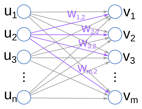
The “charge” accumulated at each neuron is some number between 0 and 1 (when we use the logistic function $\sigma$ for activation). Each weight component determines how much of that charge is passed along to influence downstream neurons. Finally, each neuron has a particular “bias” that determines how easy or difficult it is to activate that neuron generally—this is determined by the vectors $b_i$.
This kind of network is called “feed forward” because signals only propagate forwards in this network. For example, in the diagram above, charge can only flow from the $u$s to the $v$s, not backwards. It is also called “fully connected” because every neuron in each layer has a connection to each neuron in the subsequent layer. (Note that after training our network, if the $W_{i,j} = 0$, then this is equivalent to having “no connection”.)
Of course, there are many divergences both biological and algebraic between what’s going on in the artificial neural network we have constructed in this post and a true biological neural net. For one thing, biological neurons are quite a bit more complicated than this primitive approximation.
Despite (or perhaps because of) the inaccuracy, the name “neural net” stuck, and we are left with it today. Next time, we’ll take a closer look at how neural nets work and what kinds of functions they can and can’t model.
Special thanks to Eric Z., Honghao G., and Alex S. for their comments on this series!