Everything I know about Deep Learning (III)

Written on December 24, 2021

What is deep learning? How does it work? Why does it work? This is part 3 of a 3 part series on deep learning. This post looks at why deep learning works. You can find part 1 here and part 2 here.

The goal of this post is to take a stab at answering why deep learning works. But, disclaimer! This is not well-understood! (Or at least, there are very few theorems in this space so far.) In this post, I’ll try to answer this question in three ways: first, with the classical treatment of neural nets as universal approximators; second, by talking about some pecularities of gradient descent when applied to neural nets specifically; and finally by elaborating on some properties of neural nets we explored in the previous post. It is perhaps too ambitious to conclusively answer why neural nets work, but my goal is that, by the end of this post, you will at least believe it is not surprising that they work.

Universal approximators

What does it mean to say that deep learning works? In a qualitative sense, I mean that neural nets seem to do a good job at many of the tasks we use them for. But how do we quantify “good at a task”? It’s helpful to think of this as a kind of programming problem: we want to produce a program that returns a particular set of outputs when given some set of inputs (say, “this is a cat” when shown a picture of a cat). That is, we are trying to learn an unknown function.

In the first part of this series, we used this perspective to frame machine learning as a function approximation problem: suppose you have some collection of input-output pairs ${(x_i,y_i)}$ and you want to construct a function $f$ (the “model”) such that

\[f(x_i) \approx y_i\]

for each $i$. We can make the $\approx$ more precise by choosing a “loss function”, that is, a way to measure how wrong our function is on the given set of inputs. For example, when the $y_i$ are real numbers, we might choose the mean squared error

\[\mathcal{L}_{MSE}(f; x,y) = \frac{1}{N} \sum_{i=1}^{N} (y_i - f(x_i))^2\]

(and we saw that in this case, the mean squared error emerges naturally from the assumption that the errors of the model follow a Gaussian distribution.)

Often the implicit assumption in this setup is that the $x_i$ and $y_i$ are samples drawn from some spaces $X$ and $Y$, and that there is some unknown, perfect function $g$ that actually satisfies $g(x) = y$. For example, $X$ might be the space of all 128x128 pixel color images, and $Y$ might be the labels “contains a cat” and “does not contain a cat”. Then the function $g$ identifies whether a given image in $X$ contains a cat or not.

Now imagine that we have constructed our model function $f$. How do we tell how close we are to the “true” function $g$? For one thing, hopefully our loss function $\mathcal{L}$ has $g$ as its global minimum. Another approach comes from functional analysis: A function $f$ belongs to the space $L^{p}(X)$ if the $p$th root of the integral of the $p$th power of its absolute value is Lebesgue integrable. When $p = 2$, the collection of such functions forms a Hilbert space, so this is a natural choice to use when comparing functions. We say that a particular class of functions is dense in $L^{2}(X)$ if, for any function $g \in L^{2}(X, \mathbb{R})$ and every $\varepsilon > 0$, there exists a function $f$ such that

\[\sqrt{ \int_{X} \left|g(x) - f(x) \right|^{2} dx} < \varepsilon\]

The Universal Approximation Theorem says that neural nets are dense in $L^{p}(\mathbb{R}^{n}, \mathbb{R}^{m})$. This means that if we pick (almost) any function $g$, we can always find a neural net which is within $\varepsilon$ of that function for any nonzero choice of $\varepsilon$, that is, we can always approximate $g$ with a neural net with an arbitrarily small error.

Why are neural nets universal approximators?

The actual proof of the universal approximation theorem isn’t awful, but it is a little too involved for this blog post (you can read it here if you’d like). But, for completeness, I’ll attempt to sketch some intuition for why you might believe this to be true. Let’s restrict our attention to just functions $\mathbb{R} \rightarrow \mathbb{R}$ (that is, real-valued univariate functions). Let’s also assume that step functions are dense in $L^{2}(\mathbb{R},\mathbb{R})$ (if you ever computed an integral via the limit of a sum, you likely already believe this fact).

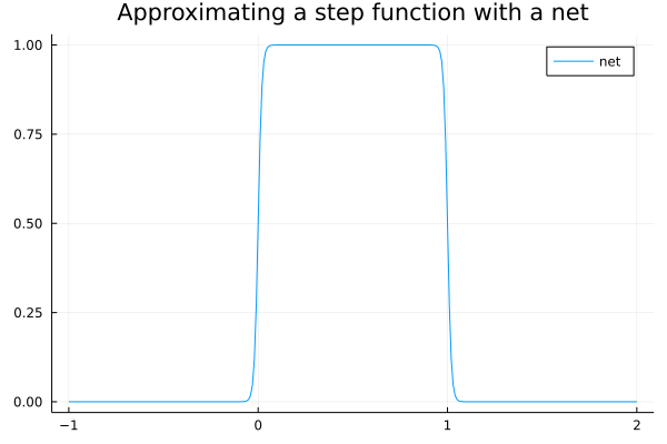
Now I will show that it is possible to approximate a step function to an arbitrary degree of accuracy with a neural net. Start with the step function

\[f(x)=\begin{cases} 1 & 0\leq x\leq1\\ 0 & \text{otherwise} \end{cases}\]

Consider the following neural net with sigmoid activation function:

\[f(x) = W_2 ( \sigma ( W_1 x + b_1)) + b_2\]

where

\[W_{1}=\left[\begin{matrix}\lambda\\ -\lambda \end{matrix}\right],\] \[b_{1}=\left[\begin{matrix}0\\ \lambda \end{matrix}\right],\] \[W_{2}=\left[\begin{matrix}1 & 1\end{matrix}\right],\]

and $b_{2} = -1$.

This is a neural net with one hidden layer (consisting of two neurons). Recall that $\sigma(x) \rightarrow 0$ as $x \rightarrow -\infty$ and $\sigma(x) \rightarrow 1$ as $x \rightarrow \infty$. As $\lambda \rightarrow \infty$, this net approaches the step function $f$. Here is a plot for $\lambda = 100$:

Once we’ve approximated one step function, we can easily add another to our net by adding additional neurons to the hidden layer. For example:

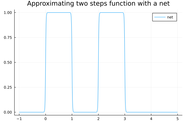
is a plot of the neural net

\[f(x)=\left[\begin{matrix}1 & 1 & 1 & 1\end{matrix}\right]\sigma\left(\lambda\left(\left[\begin{matrix}1\\ -1\\ 1\\ -1 \end{matrix}\right]x+\left[\begin{matrix}-a\\ b\\ -c\\ d \end{matrix}\right]\right)\right) - 2\]

for $\lambda = 100$, with $a=0$, $b=1$, $c=2$, and $d=3$. (The values $a$, $b$, $c$, $d$ of the bias vector $b_1$ control the extents of the step function; try varying these to see how the step functions move around.) The values of $W_2$ and $b_2$ control the “heights” of the step functions.

Because we can approximate arbitrary linear combinations of step functions using a neural net, and linear combinations of step functions are dense in $L^2(\mathbb{R})$, so too are neural nets.

So there you have it. Neural nets are universal approximators.

Sounds pretty powerful, right? Except that it turns out that lots of things are dense in $L^{2}$, in a kind of boring way: As mentioned above, linear combinations of step functions are dense in $L^{2}$, and it turns out that even polynomials are dense in $L^{2}$. And, the fact that a neural net exists which approximates your function $g$ to an arbitrarily small error doesn’t actually help you find such a function.

Recall that we actually find our neural nets through gradient descent. Is there anything special about gradient descent and neural nets?

Gradient descent is weird in high dimensions

The usage of gradient descent to train neural nets is borne out of necessity: a neural net with many large hidden layers may have a huge number of free parameters. For example, the popular (ro)BERT(a) language model from 2019 has 340 million free parameters in its “large” variant, and newer models such as OpenAI’s GPT-3 have even more than that. Gradient descent has the advantage that it is one of the only (perhaps even the only? I am not sure) numerical optimization techniques that scales well to high dimensions. Three factors make this possible:

1. In contrast to other gradient-based techniques like Newton’s method, gradient descent does not require computing a Hessian matrix (which scales $\mathcal{O}(n^2)$ with the number of free parameters.)
2. In contrast with gradient-free methods like simulated annealing, the number of samples needed to saturate the search space also doesn’t explode as the dimension of the parameter space increases.
3. As discussed in the previous post, when a function is constructed by composing smaller functions whose derivatives are known analytically, backpropogation allows us to calculate gradients of that function with a very minor computational overhead.

The last point is particularly important: if, instead of using backpropogation, we computed the gradient by numerical approximation, gradient descent would still be extremely slow.

But it’s surprising that neural nets trained by gradient descent seem to work well because gradient descent kinda sucks!

In particular gradient descent when applied to non-convex optimization problems is easily trapped in local minima and can take a long time to converge. Nevertheless gradient descent seems to be very effective at training neural nets.

Why is this?

We are now venturing into an area that is still not well understood in the community, so what follows is a guess rather than a rigorous result.

First, consider gradient descent on a non-convex surface in one dimension. If there’s a local minima, the loss surface might look something like this:

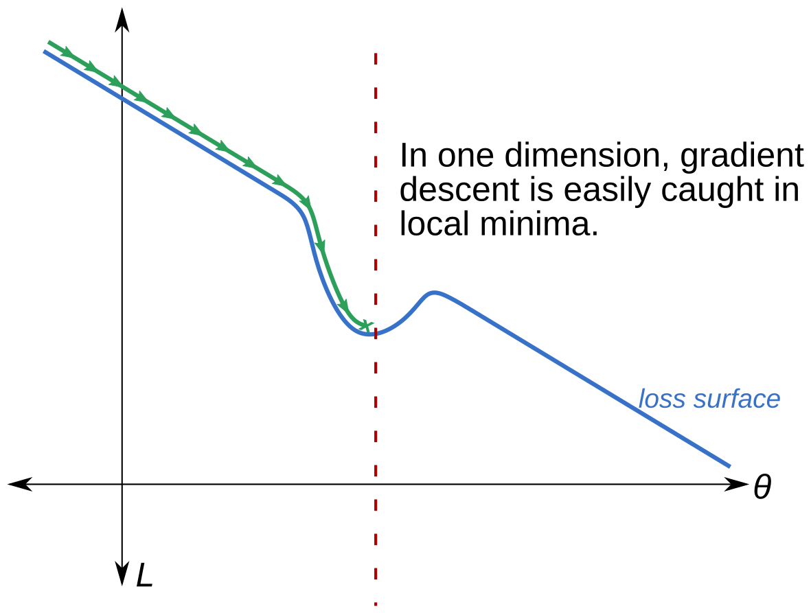
Here, $\theta$ denotes the (single) free parameter of our model, and $L$ the value of the loss function. If we initialize our model randomly (that is, pick $\theta$ at random), and there is only one local minimum, we have essentially a 50% chance of getting stuck in the local minimum depicted: if the starting point $\theta_0$ is to the left of the red line, then we’re stuck; if it’s to the right, then we can continue on our merry way.

Now suppose we add another dimension to this problem, that is, our model has two parameters. Then there are two types of local minima we can encounter: those with finite extent (depicted below), and those with infinite extent in some dimension. Let’s consider the finite-extent case first.

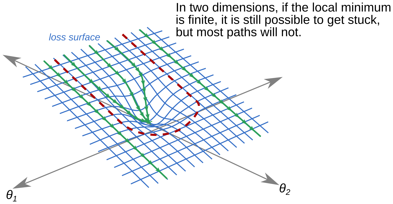
Above I have again drawn the loss surface, with a red dashed line demarcating the region where gradient flow lines will get stuck in the local minimum. In contrast to the one-dimensional case, if we pick our starting point at random, we now have a better than 50% chance of not getting stuck in the local minimum. This is of course dependent on how you initialize your starting parameters, but let’s assume for simplicity that we are picking our starting point from a multivariate normal distribution with mean zero and the identity matrix as covariances.

And, although it is now much harder to draw, we can repeat this picture in dimensions 3 and up. Each additional dimension decreases the probability of picking a starting point whose gradient flow line leads into the local minimum. Thus, in very high dimensions, it’s quite challenging to get stuck in a local minimum using gradient descent.

This analysis assumes that the local minimum has finite extents (e.g. in the two-dimensional case above, it looks like a dip instead of an infinite trough along the $\theta_1$ axis). In order for my claim to be true, it would need to be the case that most local minima are not infinite in extent in most dimensions. (In, say, 100 dimensions, a minima which is infinite in extent in 3 dimensions still leaves us with 97 dimensions where the claim holds true.)

And except in the most degenerate problems, this feels to me like it should be true? If you have a 100-million-dimensional parameter space, it should be difficult for real-world data (which invariably contains noise) to generate a local minimum which blocks gradient descent for every free parameter. And, if you have 100 million free parameters, it’s probably okay if a fraction of them do get trapped in local minima along the way; the remaining degrees of freedom should still be enough for you to model the function you want.

Nets with ReLU activations are piecewise linear

We actually proved this fact last time, but I think it’s relevant to answering why nets work as well as how. To briefly recap: one of the most common activation functions in deep learning is the “rectified linear unit”, defined by

\[\text{relu}(x)=\begin{cases} x & x\geq0\\ 0 & x<0 \end{cases}\]

This is popular in part because its gradient is just a step function (0 when $x < 0$, 1 when $x > 0$ ), which makes computing gradients particularly easy. But this choice of activation function also has an important consequence for how a net will behave: neural nets with ReLU activations are piecewise linear in their inputs.

An example of this can be seen below:

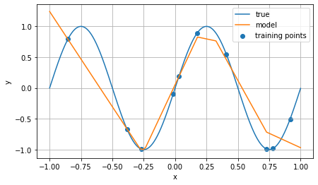
This is a plot of the output of a net (with ReLU activation) trained using only the 10 blue points; the line in blue is a sine curve, and the orange line is the net’s predictions for all points on the range from -1 to 1. The key point here is that, for out-of-sample data (inputs other than the blue points), the net linearly interpolates between the hinges that it learned during training.

Thus, one important reason why a neural net works (in the sense of, why are its predictions good) is that most data we encounter in the real world is at least locally linear, so predicting a novel value by linearly extrapolating from nearby known values is often an effective prediction technique—and this is essentially what neural nets do. In fact, because they must be differentiable almost everywhere (or more specifically, because they are chains of affine transformations and nonlinear differentiable activation functions), neural nets are constrained to be continuous functions. Note that linear extrapolation (and even continuity) is not the typical behavior of many other common modeling techniques (e.g. decision trees).

Where do nets work? Where don’t they work?

The analysis above guides us toward the sorts of problems that deep learning is suitable for. These are problems which…

• Are easily rephrased in terms of function optimization;
• Have outputs at least locally continuous with respect to the inputs (i.e., if I change an input $x_i \mapsto x_i + \varepsilon$ for some small $\varepsilon$ the output shouldn’t change that much)
• Have data available for training which reasonably captures the desired behavior (and for which linear extrapolation for novel inputs is appropriate)

Given a problem with these properties, the recipe for building a net is simple:

1. Split your data into representative training and validation sets
2. Create the largest network you feasibly can (to ensure that you are not limited in the functions you can approximate, and to help avoid local minima)
3. Initialize your net’s parameters to some random point in parameter space
4. Train iteratively using gradient descent on the training subset until you start to see performance degradation on the validation set

Now consider some of the most prominent successful applications of nets:

Image recognition is one of the first major successes. This is an area where, thanks especially to social media, there is a large amount of data available (even if most of it is unlabeled), as well as a highly curated labeled training set (ImageNet). Moreover, images are statistically stationary over a human lifetime: if a picture contains a dog in 2011, that same picture will still contain a dog in 2021, and in 2031. (Maybe in 3021 language will have changed—but maybe also grids of pixels will not be the electronic medium of choice for images.) Given these features, it is reasonable to believe that some function exists which maps a matrix of pixels to an image label, even if writing such a function by hand is very difficult. And, it is easy to validate a candidate for such a function just by inspecting its outputs. Taken together, this means we should expect image recognition to be a great use case for nets—maybe even the ideal one!

Language models like [GPT-n are another area where, depending on the task, nets can be very capable. Unlike image recognition, however, there is not an obvious way to “label” text data. Instead, neural language models are typically trained to predict the probability of a given word following some selection of text (such a model may predict a 99% probability that the phrase the quick brown is followed by fox, for example). Language models are optimized for this criterion in part because it is trivially easy to access an astronomical amount of “labeled” text for this problem: all you have to do is scrape the internet. However, we should be careful to note that such models are optimized to solve the problem text completion (“produce the most probable English text following a given prompt”), which tells us nothing about their performance characteristics on other language tasks (e.g. entailment).

These general characteristics of neural nets also underpin the controversy around applications like self-driving cars because of the assumptions inherent in applying nets to this class of problem. These are assumptions like:

• Driving a car is fundamentally a pattern recognition problem
• A large collection of captured and simulated data is sufficient to train a net-driven car, i.e., any new scenarios encountered can be extrapolated using only patterns observed in the training dataset
• Driving as a task can be suitably captured by an optimization criterion (or can be decomposed into subtasks that can be mapped to optimization criteria)

Depending on how you feel about these assumptions, self-driving cars may seem like a perfectly reasonable problem for nets, or it may sound insane! (Personally, I am skeptical, but would like to be proven wrong.)

One thing that should be clear by the end of this series, however, is that despite their capabilities, neural nets do not exhibit “thought” or “cognition” in any common meaning of the terms. Nets are no more (or less) capable of thought than mathematical functions are because that’s all a net is. (And this is a matter of some debate in philosophy.) I’ll close this series with a quote from Dijkstra:

The question of whether machines can think is about as relevant as the question of whether submarines can swim.

Deep learning can be a powerful tool when applied correctly. Hopefully this series has helped illustrate net’s strengths as well as their limitations.

Special thanks to Eric Z., Honghao G., and Alex S. for their comments on this series!