What's your house worth?
Over four million homes were sold in 2024, with a median sale price of $407,500 (source). That’s $1.66 trillion of residential real estate transactions in 2024 alone! And yet, house prices are notoriously difficult to predict—just ask Zillow! In this post, I’ll talk about some of the challenges in pricing illiquid assets (like homes), highlight how those challenges impact model design, and ultimately develop a fairly sophisticated house pricing model. Along the way, we’ll touch on topics like heteroskedasticity, hierarchical modeling, and Bayesian regression.
Preliminaries
Data acquisition
Before we can do any modeling, we need to get some data. There are a number of places you can go to find this data—for this post, I pulled data from redfin.com, which provides a convenient download service (accessible on the desktop site via the “Download all” button at the bottom of search results).
Note that Redfin (and other providers, like Zillow) license their data from MLS, and consequently impose certain restrictions on its usage and publication. In order to comply with those terms of use, I will not be sharing the raw data used in this post, nor can I provide any detail about the geographic locale of my query. You’ll just have to use your imagination!
Tools
For this post, we’ll be working in Julia, and leveraging a number of packages:
- DataFrames.jl and CSV.jl (for CSV parsing);
- Query.jl for querying Julia data sources;
- Assorted statistics packages: Distributions.jl, StatsModels.jl, GLM.jl, CategoricalArrays.jl;
- Turing.jl, a probabalistic programming framework;
- And, for plotting, Plots.jl and StatsPlots.jl
Data ingress and cleaning
The dataset I pulled from Redfin contains a number of fields, but there are only a few we are interested in:
- Price - the sale price of the home;
- Sold date - the date of the sale;
- City - the municipality the home is located in;
- Square feet - the size of the home (in square feet);
- Property type - one of “single family residential”, “condo/co-op”, or “townhouse”;
- Beds - the number of bedrooms of the home; and
- Baths - the number of bathrooms of the home (may be fractional)
In order to build a model off of these features, we need to ensure they are all present and reasonably-valued. This is easy to do leveraging Query.jl:
# ingest the data and clean up column names
df = DataFrame(CSV.File("my-house-csv-file.csv"));
rename!(df, Dict(names(df) .=> replace.(names(df), " " => "_")));
rename!(df, Dict("\$/SQUARE_FEET" => "PRICE_SQFT"));

# transform the date strings into Dates
function parse_custom_date(date_str)
    return Date(date_str, "U-d-y")
end

# parse dates, order, and drop missings
# and other invalid data
df = df |>
    @select( :PRICE, :SOLD_DATE, :SQUARE_FEET,
        :BEDS, :BATHS, :PROPERTY_TYPE, :CITY, :PRICE_SQFT,
        :LATITUDE, :LONGITUDE) |>
    @dropna() |>
    @mutate(SOLD_DATE = parse_custom_date(_.SOLD_DATE)) |>
    @filter(_.SQUARE_FEET > 1) |>
    @orderby(_.SOLD_DATE) |>
DataFrame;
Note that the @dropna() is potentially very destructive—a more thorough treatment would address missingness (perhaps those fields are missing for a reason?), but in my case only a handful of properties were missing these fields, and usually for sensible reasons (for instance, some records are vacant land).
Note also that our categorical fields (“CITY”, “PROPERTY_TYPE”) are currently still treated as strings—to fix this, we need to cast them to categorical arrays:
df.PROPERTY_TYPE = categorical(df.PROPERTY_TYPE);
df.CITY = categorical(df.CITY);
I’m primarily interested in single-family homes (what can I say, I’m a dad with young kids), so I’m going to make that the base case for my PROPERTY_TYPE categorial array:
levels!(df.PROPERTY_TYPE,
    ["Single Family Residential", "Condo/Co-op", "Townhouse"])
We’ve now got a reasonably clean dataset to work from.
Exploratory data analysis
Before diving into model building, let’s spend a minute to take a quick look at our data and see if we can tease out some relationships between our covariates. Exploratory data analysis, even on a toy problem like this, can be very valuable. For one thing, the relationships between our covariates and the response will help us sanity check the coefficients on our models.
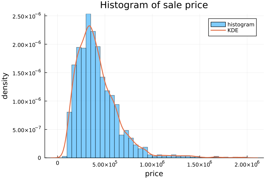
Price distribution
Before we look at any of the covariates, it is useful to ask the question “how are prices distributed?” Prices are non-negative (outside of certain exceptional circumstances, house prices generally cannot sell for less than 0 dollars) but uncapped (a house can be arbitrarily expensive). A good starting point for this kind of variable is a log-normal distribution. We can check how closely our data matches this distribution using a Q-Q plot:
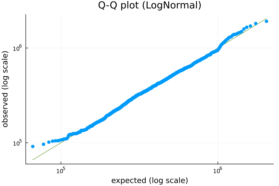
A Q-Q plot compares the quantiles of two distributions. In this case, we’re comparing the empirical quantiles of our price data against the predicted quantiles if the data followed the best-fitting log-normal distribution. I’ve plotted the data on a log scale so that observations are more evenly distributed visually (otherwise, the outlying high prices would be very far away from the rest of the data).
A perfect match against the log-normal distribution would have all of the observations on the green “y = x” diagonal. This plot is not perfect, but it’s a pretty close fit. At very low prices, the observed quantiles are larger than expected, i.e., the observed price at, say, the 3rd percentile is larger than would be expected if this perfectly matched a log-normal distribution. This suggests that there’s a higher “floor” on prices than would be expected from a log-normal distribution.
This mismatch disappears rapidly, and otherwise the prices seem to very closely follow a log-normal distribution.
Prices over time
First, let’s look at house prices over time.
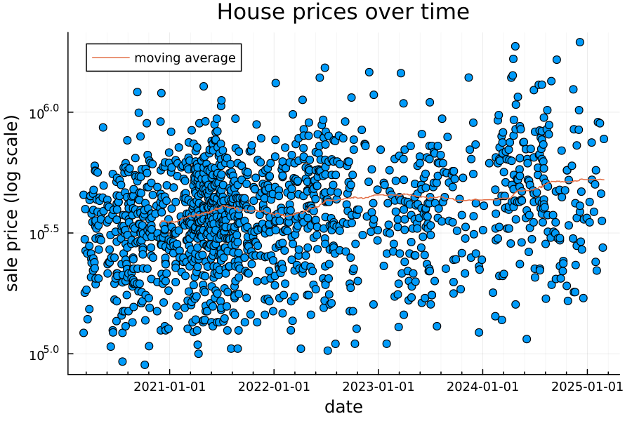
Note that the price is on a log scale, and the moving average is over the past 250 observations. It looks like there’s a weak positive relationship, suggesting home prices in this area have on average been slowly increasing over the past 5 years.
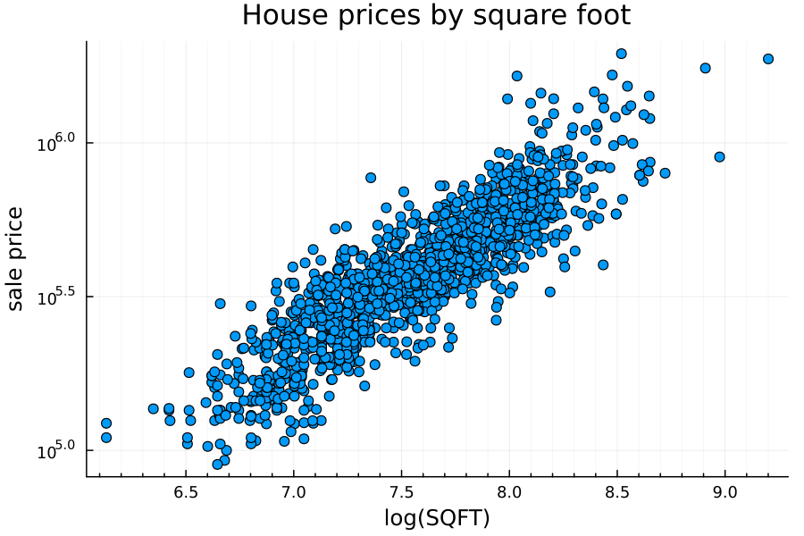
Price vs square footage
A much stronger determinant of house price is the square footage of the home. Because both home price and square footage has a long right tail, I’ve plotted both axes on a log scale.
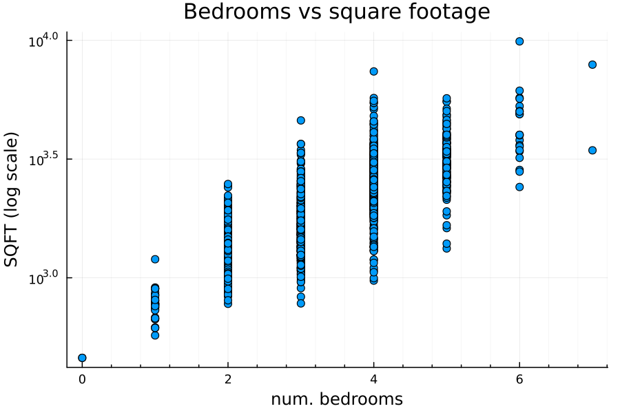
Price vs number of bedrooms
There’s a positive relationship between number of bedrooms and home price:
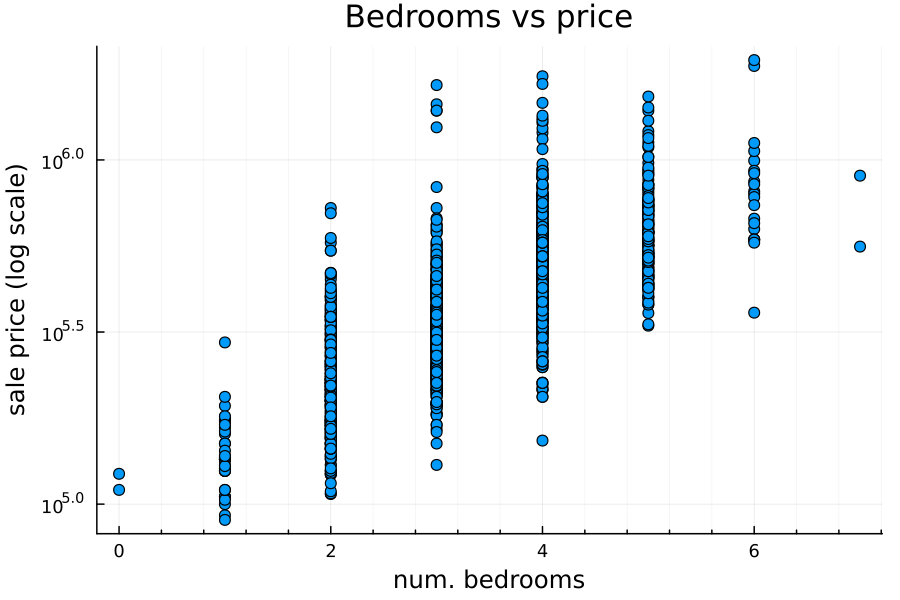
However—and this will be important later!—there is also a positive relationship between number of bedrooms and square footage:
Location vs price
There’s also a relationship between the location and price. Below, I’ve plotted the moving average price over time for each city in my dataset:
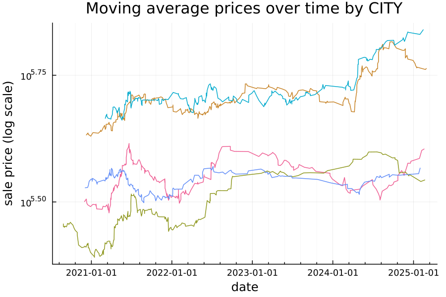
For those not quick with exponenents (such as myself), the gap between $10^{5.5}$ and $10^{5.75}$ is about $246,000, so there’s a difference of almost a quarter of a million dollars between the mean sale price of homes in the teal city and homes in the brown city. This suggests (unsurprisingly) that location is likely to be a relevant feature for this analysis.
Model construction
So far, the relationships we’ve seen in the data are broadly intuitive: more square footage = higher price, more bedrooms = higher price, more bathrooms = higher price (not plotted), and prices have been broadly increasing over time. Let’s see if those are reflected in our model.
To begin, we need to create a “model matrix”—a processed dataset we can run our model through. Julia’s StatsModels.jl package provides a convenient framework for doing this.
We’ll do two bits of feature engineering: because of the aforementioned long right tail on square footage, we’re going to use the log of the square footage rather than the square footage directly. (Put another way, we’re going to assume that square footage follows a log-normal distribution.) We’ll also convert the dates into a “years since”, where the most recent sale occurs at time 0 and the oldest at about time 5 (5 years).
Xy = let
    max_date = maximum(df.SOLD_DATE)
    df |>
        @mutate(LOG_SQFT = log(_.SQUARE_FEET)) |>
        @mutate(DT_YRS =
            Dates.value(max_date - _.SOLD_DATE) / 365) |>
        @select(:PRICE, :DT_YRS, :LOG_SQFT,
            :BEDS, :BATHS, :PROPERTY_TYPE, :CITY) |>
    DataFrame
end
Here’s a matrix of input features:
X = modelmatrix(
    @formula(PRICE ~ 1 + DT_YRS + LOG_SQFT + BEDS
    + BATHS + PROPERTY_TYPE), Xy)

y = Xy.PRICE
This should return a matrix like this:
1491×7 Matrix{Float64}:
 1.0  4.9863     7.82724  5.0  2.5  0.0  0.0
 1.0  4.9863     7.00307  2.0  2.0  1.0  0.0
 ⋮                                  ⋮
 1.0  0.0109589  6.89871  2.0  2.0  0.0  0.0
 1.0  0.0        8.29455  5.0  4.0  0.0  0.0
Note that this is one case where it matters what order the levels are in in our categorical array PROPERTY_TYPE: modelmatrix does a one-hot encoding of the categorical features, treating the first level as the base case.
For my analysis, I’ve treated single-family homes as the base case, and then the other two indicator variables correspond to “condo/co-op” and “townhouse”, respectively.
To create train and test splits, I’m going to set aside about 250 observations for out-of-sample testing, and use the remainder for training. I’m doing this by recency—I don’t want there to be any leakage of future information into my model—so I’ll just take the most recent 250-ish sales:
X_train, X_test = X[1:1200,:], X[1201:end,:]
y_train, y_test = y[1:1200], y[1201:end]
Classic OLS linear regression
As a starting model, let’s create a simple ordinary least squares (OLS) linear regression model. (This uses the GLM.jl package.) Just like square footage, home prices follow a log-normal distribution, so we will fit this model on the log of the house prices. That is, the final model will look something like:
\[\hat{y} = \exp({X \beta})\]or, alternatively,
\[\log(y) \sim N(X \beta, \sigma)\]where $y$ is the sale price, $\beta$ is our model’s coefficients, $X$ the input matrix, and $\sigma$ the standard deviation.
Here’s the model:
ols_regr = lm(X_train, log.(y_train))
and the resulting coefficient matrix:
| Coef. | Std. Error | t | Pr(> |t|) | Lower 95% | Upper 95% | |
|---|---|---|---|---|---|---|
| intercept | 8.24369 | 0.164418 | 50.14 | <1e-99 | 7.92111 | 8.56627 |
| DT_YRS | -0.103076 | 0.00647597 | -15.92 | <1e-51 | -0.115782 | -0.0903707 |
| LOG_SQFT | 0.632227 | 0.0246884 | 25.61 | <1e-99 | 0.58379 | 0.680665 |
| BEDS | -0.0199786 | 0.00963452 | -2.07 | 0.0383 | -0.0388811 | -0.00107605 |
| BATHS | 0.116563 | 0.0100247 | 11.63 | <1e-28 | 0.0968948 | 0.136231 |
| IS_CONDO | -0.405853 | 0.020437 | -19.86 | <1e-75 | -0.445949 | -0.365756 |
| IS_TOWNHOUSE | -0.205446 | 0.0164896 | -12.46 | <1e-32 | -0.237797 | -0.173094 |
The table above includes the value of the coefficient as well as the t-score (the value of the coefficient divided by the standard error), and a confidence range on the coefficient.
The intercept is 8.24, corresponding to a price of $3,803 (apparently, the going price in March 2025 for a single-family home with zero beds, zero baths, and occupying 1 square foot).
With the exception of BEDS, the t-scores for all of the features are all quite extreme, suggesting a strong relationship between the log price and that corresponding covariate.
The t-score for BEDS is somewhat lower, at just -2.07, suggesting a comparatively weaker relationship.
On top of that, it’s negative, despite a strong positive correlation between price and number of bedrooms.
What gives?
The answer lies in our choice of covariates: recall that bedrooms and square footage are strongly correlated.
This means that, after adjusting for the impact of square footage, the remaining impact of number of bedrooms is actually weakly negative. The intuition for this is straightforward: holding all else constant (including the size of the house), adding more bedrooms will decrease the value of the home.
Another important point to remember when looking at these coefficients is that they are multiplicative on the predicted price, not additive. So, for instance, the “condo” effect is a multiplier of $\exp(-0.406) = 0.666$, i.e., a condo of the same square footage, number of bedrooms, and number of bathrooms is predicted to sell for only 67% the price of the equivalent single-family residence. (The “townhouse” penalty is somewhat milder at 81%.)
The final coefficient to highlight is DT_YRS, the time since the sale.
Our choice of coordinates for time make this a little bit nonintuitive—recall that DT_YRS is 0 in March 2025 and increases linearly to 5 in March 2020.
Therefore, the coefficient of $-0.103$ suggests that, after controlling for other factors, home prices have been increasing by a factor of $\exp(0.103076) = 1.109$ (i.e. 10.9% a year) on average each year since 2025.
Model evaluation
We deliberately left out approximately 250 observations from our training set to use for out-of-sample evaluations. How well does this model perform on these observations? To answer this, let’s compute the mean absolute error (MAE):
mean(abs.(y_test .- exp.(predict(ols_regr, X_test))))
# returns 83188.85
That is, the mean absolute error of the model is about $83k. This seems like a big number (and it is), but remember that this model operates in log space, and prices appear to follow a log-normal distribution:
$83k is not a huge error on a multi-million-dollar house. It can be more informative to look at the MAE of the log prices (equivalent to the percentage error on the price). In this case, the MAE of the log price is 0.152, which is about 16.5%.
Spot checking the residuals of the ordinary least squares model, the results look reasonable:
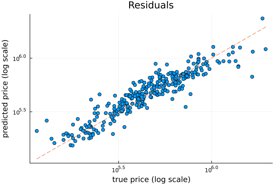
(As a reminder, the dashed line is “x = y”, i.e., the closer a model’s predictions are to that line, the better fit the model is.)
Bayesian linear regression
Note that ordinary least squares regression imposes assumptions on our data: for instance, that the errors of the regression are independent and identically distributed with mean 0. To build a more sophisticated model, we may need to weaken some of these assumptions. However,
To try a more sophisticated approach, let’s utilize the probabalistic programming framework Turing.jl. Turing provides a framework for performing Bayesian inference with an intuitive model specification that closely resembles mathematical notation (we’ve discussed Turing.jl before).
The advantage of this approach is in its flexibility: we need only specify the prior distributions we believe the parameters, covariates, and responses to be sampled from, and then the Hamiltonian Monte-Carlo (HMC) sampling will take care of the rest for us.
Let’s start just by re-implementing the linear regression above.
@model function bayes_lin_regr(X, y)
    # n = number of observations
    # p = number of covariates
    n, p = size(X)
    # coefficients are drawn from a multivariate
    # normal distribution
    β ~ MvNormal(zeros(p), 10.0 * I)
    σ ~ truncated(Normal(0, 5), 0, Inf)
    # the expected value is the product of the coefficients
    μ = X * β
    for i in 1:n
        # each observation is drawn from a normal
        # distribution with mean μ[i] and std dev σ
        y[i] ~ Normal(μ[i], σ)
    end
end
Create an instance of this model by passing in the training set and the response:
model = bayes_lin_regr(X_train, log.(y_train))
To actually estimate the model parameters, we need to estimate the posterior distributions on our parameters. We’ll do this using the No U-turn sampler (NUTS):
# sample for 5000 steps
chain = sample(model, NUTS(), 5000)
Here are the resulting coefficients:
| coeff | mean | std | mcse | 2.5% | 97.5% |
|---|---|---|---|---|---|
| intercept | 8.2188 | 0.1662 | 0.0039 | 7.8879 | 8.5383 |
| DT_YRS | -0.1027 | 0.0066 | 0.0001 | -0.1157 | -0.0896 |
| LOG_SQFT | 0.6358 | 0.0251 | 0.0006 | 0.5873 | 0.6847 |
| BEDS | -0.0204 | 0.0099 | 0.0002 | -0.0398 | -0.0008 |
| BATHS | 0.1158 | 0.0102 | 0.0002 | 0.0957 | 0.1357 |
| IS_CONDO | -0.4046 | 0.0207 | 0.0004 | -0.4447 | -0.3643 |
| IS_TOWNHOUSE | -0.2049 | 0.0164 | 0.0003 | -0.2373 | -0.1732 |
| σ | 0.1787 | 0.0037 | 0.0001 | 0.1717 | 0.1861 |
The coefficients found via our sampling process are quite similar to those found via the OLS linear regression model. In addition to the values of the coefficients, we can also get the empirical distribution observed for each coefficient during the sampling process.
For example, to plot the distribution of the coefficient of DT_YRS (β[2]):
plot(title="DT_YRS - density", fmt=:png, dpi=150)
density!(chain[:, Symbol("β[2]"), 1], label="")
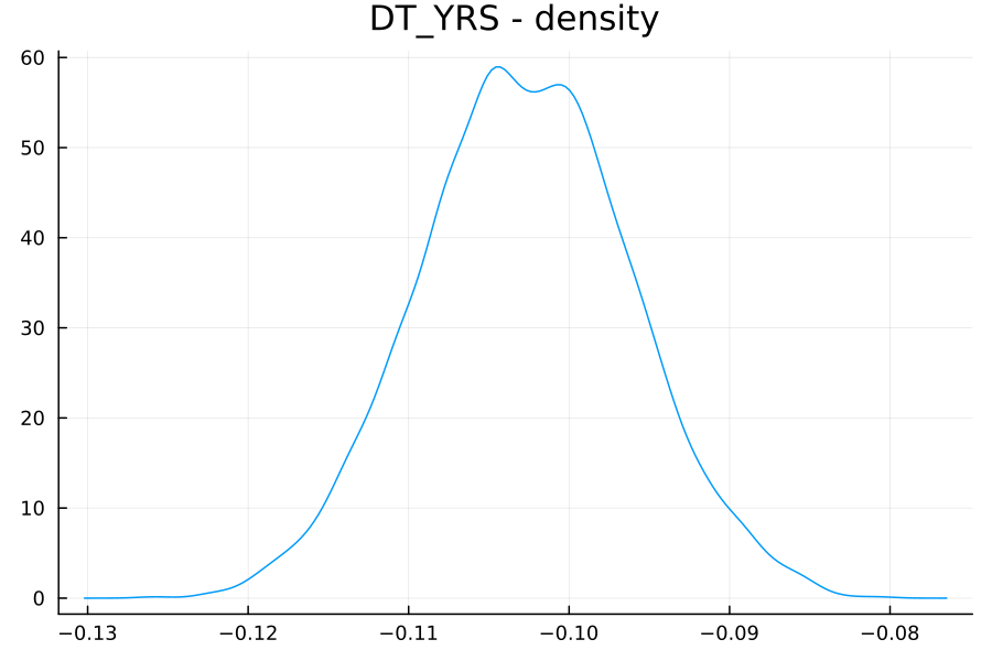
Note that this empirical density is not a classic normal distribution (in contrast to what OLS would have predicted), although it is close to one.
Model evaluation
Predictions with a Bayesian model are produced via a similar process to the HMC sampling: in this case, the response is simply treated as another set of parameters to be estimated.
In Turing, unknown parameters are specified by missing elements, so we supply an array of missings to the model invocation.
The predict function also expects to get the chain of samples we produced earlier to estimate our parameters.
preds = predict(
    bayes_lin_regr(X_test, missings(Int64, length(y_test))),
    chain)
Note that the result of this function is also a chain—so, for each prediction we also get an empirical distribution. For example, the model’s predicted distribution for the 13th out-of-sample observation is:
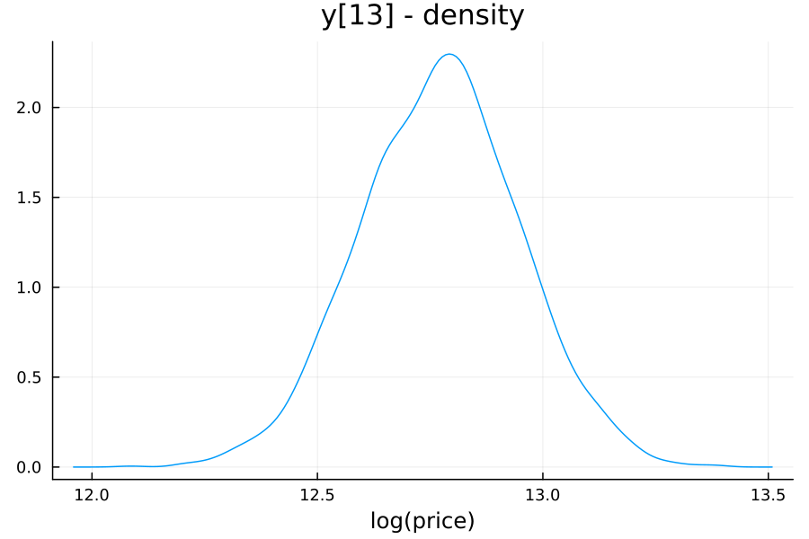
In this case, the home in question is a 2100 square foot condo with 2 bedrooms and 2.5 baths, sold in 2023, with an estimated price between 248k and 499k. Incidentally, the home sold for 725k, so neither the classical or Bayesian linear regressions were particularly accurate.
The mean absolute error can be computed by
mean(abs.((y_test) .- exp.(mean(preds.value.data, dims=1)[1,:,1])))
which returns $83,108. This number is close to (and in fact slightly lower than) the MAE of our OLS regression, but we can still do better.
Log-normal Bayesian regression
First, let’s correct the distribution: we are interested in modeling the price itself, not the log price, so it is natural to sample this from a log-normal distribution. The modification is minimal:
@model function lognorm_regr(X, y)
    n, p = size(X)
    β ~ MvNormal(zeros(p), 10.0 * I)
    σ ~ truncated(Normal(0, 5), 0, Inf)
    μ = X * β

    y ~ MvLogNormal(μ, σ * I)
end

model = lognorm_regr(X_train, y_train)
chain = sample(model, NUTS(), 5000)
The resulting coefficients are, unsurprisingly, very similar to before:
| coeff | mean | std | mcse | 2.5% | 97.5% |
|---|---|---|---|---|---|
| intercept | 8.2300 | 0.1627 | 0.0036 | 7.9174 | 8.5565 |
| DT_YRS | -0.1030 | 0.0066 | 0.0001 | -0.1161 | -0.0900 |
| LOG_SQFT | 0.6343 | 0.0246 | 0.0005 | 0.5852 | 0.6815 |
| BEDS | -0.0203 | 0.0098 | 0.0002 | -0.0392 | -0.0009 |
| BATHS | 0.1161 | 0.0097 | 0.0002 | 0.0974 | 0.1350 |
| IS_CONDO | -0.4052 | 0.0200 | 0.0004 | -0.4438 | -0.3642 |
| IS_TOWNHOUSE | -0.2051 | 0.0162 | 0.0003 | -0.2368 | -0.1732 |
| σ | 0.1789 | 0.0036 | 0.0000 | 0.1722 | 0.1862 |
and the MAE on the out-of-sample set is $84,443—very slightly worse than our other two models. (We may at least take some small comfort in the knowledge that our model more accurately reflects the distribution of the response.)
Heteroskedasticity
We’re not done yet, though. We’re most interested in using this model for forecasting or even nowcasting: we want to estimate, today, what would a given house sell for. The housing market is nonstationary: sales occurring further in the past are therefore less informative about the current relationship between price and covariates.
One way to model this uncertainty (in a very Bayesian sense) is through heteroskedasticity: we will allow the variance of the model to vary over time, rather than remain constant. In particular, the further back in time the observation occurred, the higher the variance (i.e. the less informative) we want the observation to be.
To model this, I’m going to assume that the variance positively increases according to the following exponential relationship:
\[\sigma_{t} = \sigma_{0} e^{\alpha t}\]where both $\sigma_{0}$ and $\alpha \geq 0$.
Here’s our modified model:
@model function heteroskedastic_regr(X, y, t)
    n, p = size(X)
    β ~ MvNormal(vcat([8.16], zeros(p-1)), 10.0 * I)
    σ0 ~ truncated(Normal(0, 5), 0, Inf)

    α ~ truncated(Normal(0, 5), 0, Inf)
    σ = σ0 * exp.(α .* t)

    μ = X * β
    y ~ MvLogNormal(μ, Diagonal(σ))
end
The 8.23 intercept prior is taken from our result from OLS above.
Note that this accepts an additional argument, t, which by my convention represents how far in the past the observation occurred, measured in years.
The prior
α ~ truncated(Normal(0, 0.1), 0, Inf)
imposes a constraint that $\alpha \geq 0$
Estimate the parameters of the model as before:
model = lognorm_regr(X_train, y_train)
chain = sample(model, NUTS(), 5000)
and we find some slight changes in our coefficients:
| coeff | mean | std | mcse | 2.5% | 97.5% |
|---|---|---|---|---|---|
| intercept | 8.2279 | 0.1650 | 0.0038 | 7.9082 | 8.5524 |
| DT_YRS | -0.1029 | 0.0067 | 0.0001 | -0.1162 | -0.0896 |
| LOG_SQFT | 0.6342 | 0.0246 | 0.0006 | 0.5852 | 0.6816 |
| BEDS | -0.0197 | 0.0096 | 0.0002 | -0.0383 | -0.0005 |
| BATHS | 0.1159 | 0.0102 | 0.0002 | 0.0960 | 0.1363 |
| IS_CONDO | -0.4043 | 0.0210 | 0.0004 | -0.4445 | -0.3625 |
| IS_TOWNHOUSE | -0.2048 | 0.0167 | 0.0003 | -0.2367 | -0.1713 |
| σ0 | 0.1726 | 0.0063 | 0.0001 | 0.1587 | 0.1829 |
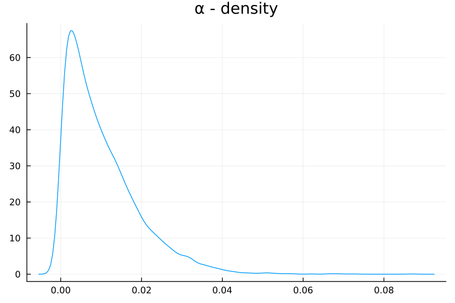
| α | 0.0103 | 0.0090 | 0.0002 | 0.0003 | 0.0326 |
The new $\alpha$ parameter has the following distribution:
The model’s inferred heteroskedasticity is plotted below:
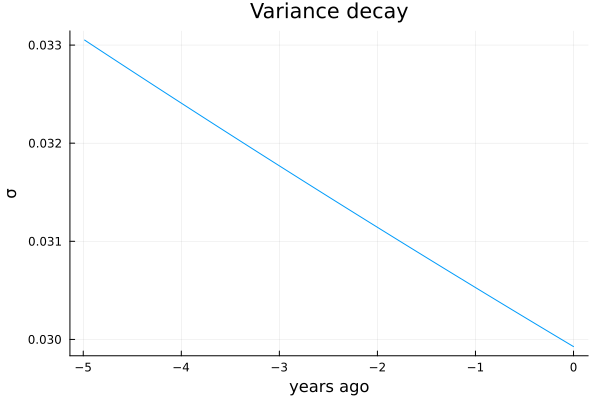
This model also has a slightly improved MAE of 84,409 compared to our previous attempt. (For those following along at home, it also does very slightly better at predicting the price of out-of-sample home 13—guessing 506k this time around.)
Hierarchical heteroskedastic log-normal regression
The number one rule of real estate (at least according to the Octonauts) is location, location, location. There are actually thirteen different cities that the data in this dataset is drawn from, and we haven’t been using that information. There are a few different ways one might incorporate this information, but because we’re already in a Bayesian mood, let’s build a hierarchical model.
In a hierarchical model, the assumption is that the data is naturally organized into a hierarchy of groups—in our case, each home belongs to a neighborhood, each neighborhood belongs to a city, each city to a county, and so forth. We want the relationships between our covariates and the response to be informed by location, but we don’t want to fit entirely independent models on each segment of our data. Instead, we’d like these models to inform each other via a global population-level model, and moreover we’d like the way that information is passed around to reflect the observations we have for that particular segment. (For example, when we have very few observations, we’d like the coefficients of our regression to more closely resemble the global coefficients, whereas segments that have many observations may be more informed by that segment’s observations.)
This dataset is a good candidate for a hierarchical model: as observed previously, there are differences in average price between cities. There are also wide differences in the number of observations seen from each city:
| City | Count |
|---|---|
| 1 | 16 |
| 2 | 2 |
| 3 | 9 |
| 4 | 15 |
| 5 | 12 |
| 6 | 4 |
| 7 | 279 |
| 8 | 347 |
| 9 | 2 |
| 10 | 288 |
| 11 | 288 |
| 12 | 4 |
| 13 | 225 |
Let’s look at two different ways to construct a hierarchical model from our existing regression.
Model 1: Intercept-only
The simplest way to introduce a hierarchy is to allow only one of our covariates (the intercept) to vary by location. In other words, the model is
\[y_{i} \sim \log N( X_{i} \cdot \beta + \lambda_{g}, \sigma_{i})\]where
\[\beta_{j} \sim N(0, 5)\] \[\lambda_{0} \sim N(0, 5)\] \[\lambda_{g} \sim N(\lambda_{0}, 5)\]Here, $\lambda_{0}$ is the global intercept, and $\lambda_{g}$ is the intercept for group $g$.
Here’s the model implementation in Julia:
# G is the group index, nG the number of groups
@model function hiearch_regr(X, y, t, G, nG)
    n, p = size(X)
    # global coefficients
    β ~ filldist(Normal(0, 5), p - 1)
    # global intercept
    λ0 ~ Normal(8.17, 3)

    # group intercepts
    λj ~ filldist(Normal(λ0, 5), nG)

    σ0 ~ truncated(Normal(0, 5), 0, Inf)
    α ~ truncated(Normal(0, 0.1), 0, Inf)
    σ = σ0 * exp.(α * t)

    μ = X[:,2:end] * β .+ λj[G]
    y ~ MvLogNormal(μ, Diagonal(σ))
end
This model results in broadly similar choices of coefficients (for instance, 0.6309 for LOG_SQFT).
However, we get an interesting distribution for $\lambda_{0}$, the global intercept:
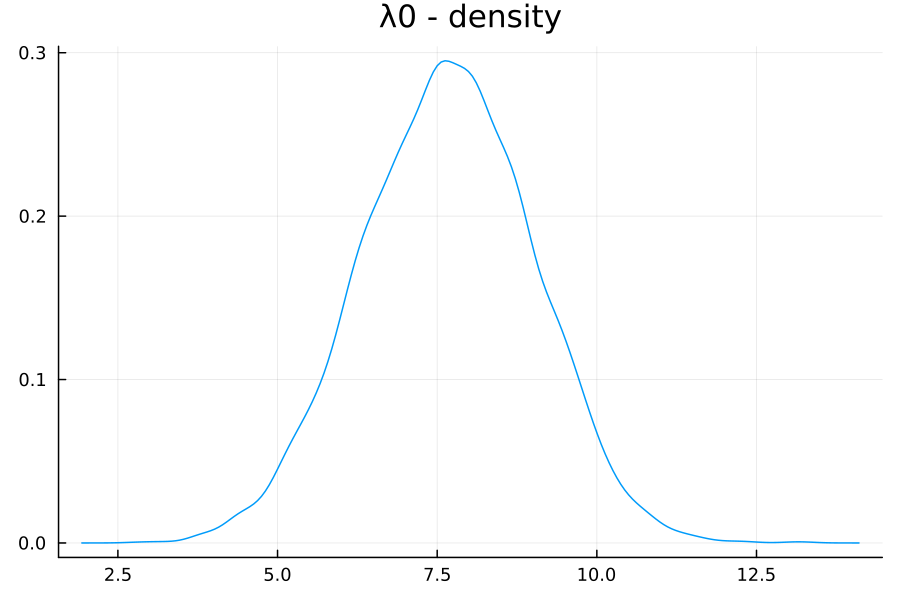
Moreover, this gives us our best MAE yet, 77493. (Home 13’s prediction is still quite a bit off, at 391k vs a true value of 725k—it’s possible that this condo is a bit of an outlier.)
Model 2: Full hierarchical
But why restrict ourselves to just a “random-intercept” model? We can extend our multilevel model to allow for a hierarchical relationship between the coefficients as well:
@model function hiearch_regr2(X, y, t, G, nG)
    n, p = size(X)
    # global coefficients
    β ~ filldist(Normal(0, 5), p)

    # group coefficients
    βj ~ filldist(MvNormal(β, 5 * I), nG)

    σ0 ~ truncated(Normal(0, 5), 0, Inf)
    α ~ truncated(Normal(0, 0.1), 0, Inf)
    σ = σ0 * exp.(α * t)

    μ = sum(X .* βj[:,G]', dims=2)[:,1]

    y ~ MvLogNormal(μ, Diagonal(σ))
end
Note that this model has more parameters to estimate than our previous regressions, and consequently is much more demanding on our sampler.
For this reason, it can be worthwhile to swap out the underlying automatic differentation engine used by NUTS from the default (provided by Zygote.jl) to one provided by ReverseDiff.jl instead.
To do this, you have to first import ReverseDiff, and then specify it as an argument to the sampler:
model = hiearch_regr2(X_train, y_train, X_train[:,2], G_train, 13)
chain = sample(model, NUTS(adtype=AutoReverseDiff(true)), 2000)
The true argument to AutoReverseDiff pre-records the tape once so that it can be re-used for a significant speedup; beware that for more sophisticated models (e.g. with branching logic), this may introduce errors.
I have also lowered the number of samples to do from 5000 to 2000, so that the computation completes in a reasonable amount of time.
(Reasonable in this case still being about 20 minutes!)
We can now look again at our intercept densities. I’ve plotted below the global density (in blue) along with the learned densities per city.
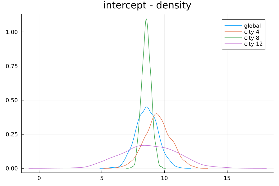
Recall that City 4 has 15 observations, City 8 has 347, and City 12 has only 4 observations. These population counts are reflected in the variances of the learned distributions: the model in particular has a very low confidence for the intercept of City 4.
A similar story plays out for the coefficent of LOG_SQFT:
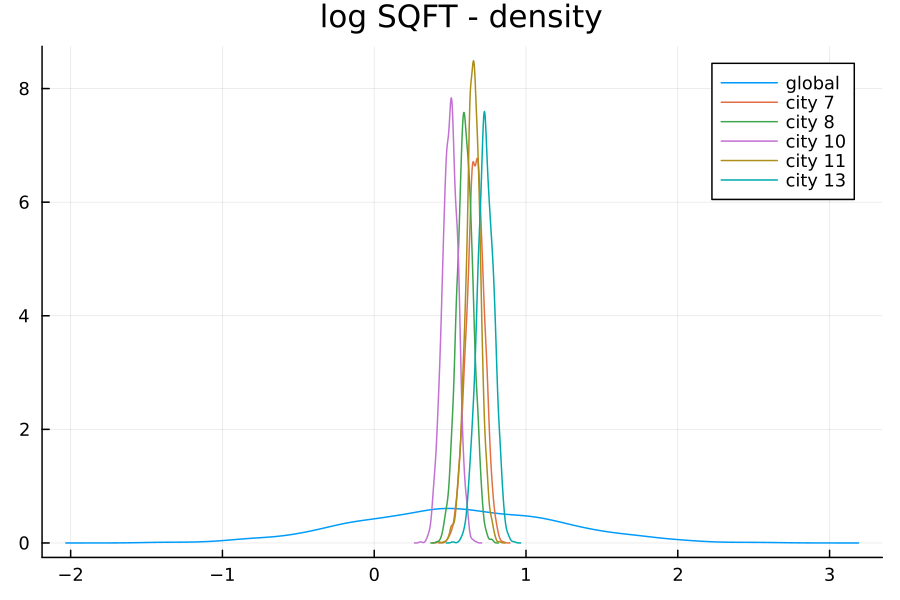
I’ve plotted above the 5 most populous cities in the dataset (each with more than 250 observations), along with the global prior. The confidence range for each distribution is quite concentrated. However, observe that each city has a distinct distribution, resulting in greater uncertainty in the global distribution.
This hierarchical model, while beating our previous linear regressions, actually underperforms the intercept-only hierarchical model on the out-of-sample dataset: its MAE is 81,552. (This is one way to tell that the numbers weren’t fudged!)
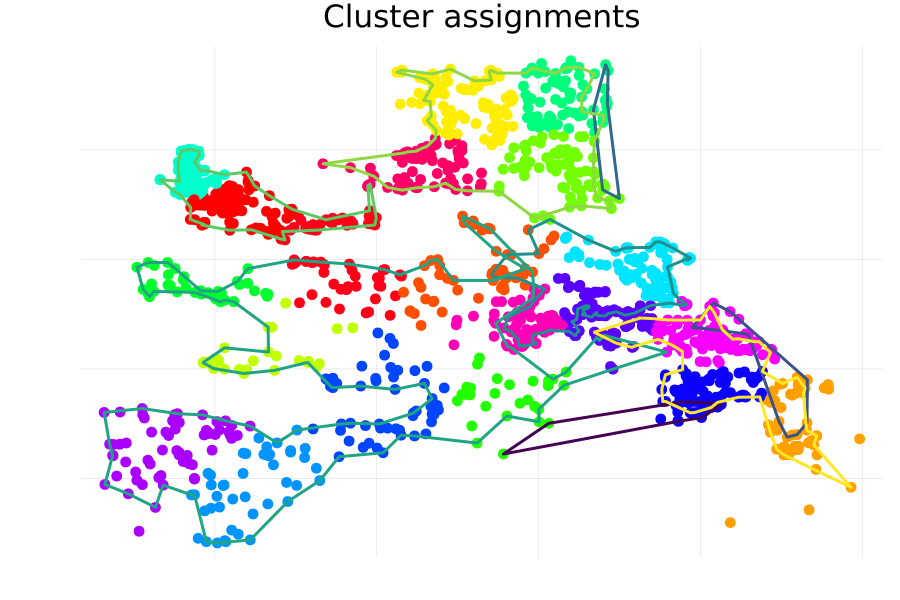
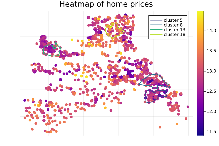
Model 3: Alternative hierarchies
One reason the hierarchical models here have not made a significant difference might be that “city” is too broad, and house prices vary geographically within each city. For instance, here is a heatmap of the log prices overlayed on top of a concave hull bounding each city region:
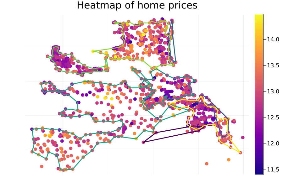
One city (the “green”-ish one starting from the lower-left of the diagram) covers a large geographical area, and there may be meaningful differences in location between properties in the southwest region as compared to those in the eastern portion. To get more granular group assignments, we could instead construct a cluster assignment using the latitude and longitude of each property.
This is easily done with Clustering.jl.
Here, I used k-means clustering with 20 cluster assignments:
clusters = let
    X = Matrix{Float64}(df |>
        @select(:LATITUDE, :LONGITUDE) |>
        DataFrame)
    X = transpose(X)
    R = kmeans(X, 20; maxiter=200, display=:iter)
    assignments(R)
end
Integrating this into our hierarchical model is essentially the same as using the “City” grouping—the only difference is we should supply the cluster index instead of the city index.
G = df.CLUSTER
G_train = df.CLUSTER[1:1200];
G_test = df.CLUSTER[1201:end];

# 20 clusters
model = hiearch_regr(X_train, y_train, X_train[:,2], G_train, 20)
There are distinctly different intercepts learned for each cluster, suggesting that geographic location does play an impact in determining the home price:
However, despite these efforts, the final performance of the model is still only about on-par with our original ordinary least squares approach:
The MAE on the out-of-sample set is in fact worse, at 86987.3 vs 83188.9.
In general, a comparison of the out-of-sample residuals between the two models shows that, although there are some cases (the green arrows) where our hierarchical model did better, on balance it is slightly worse:
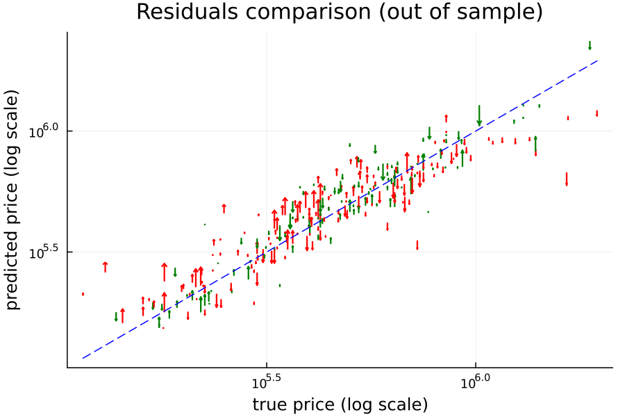
So what gives?
To get an idea of what’s going on, it is instructive to look at the in-sample performance of this hierarchical model:
The in-sample MAE is 52904.3, as compared to the OLS model’s 56461.8.
This suggests that, unsurprisingly, adding more learnable parameters to our model has improved our in-sample performance at the cost of generalization.
What happens if we add our cluster assignment as a categorical feature accessible to our OLS model?
As expected, it improves the in-sample error by quite a bit—to 50817.5.
Perhaps more surprisingly, it also improves the out-of-sample error as well, to 71730.8.
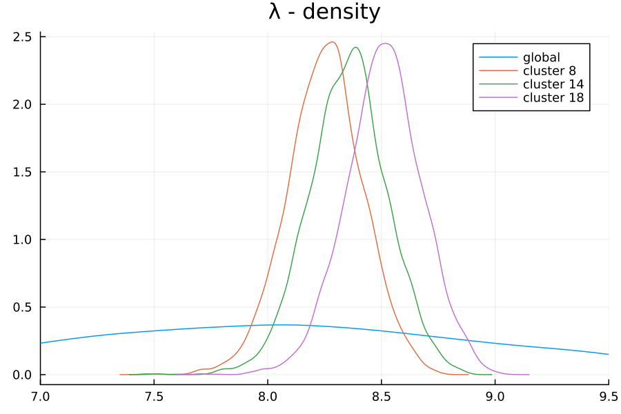
What’s more, several of the cluster assignments are statistically significant—in particular, clusters 5, 8, 13, and 18.
This is reflected both in the distributions learned by our hierarchical model (see the density plot above), as well as in the heatmap itself:
In particular, the coefficient associated with cluster 13 is -0.0933, suggesting a negative impact relative to the baseline property value for that cluster; similarily it is -0.1071 for cluster 8 and -0.1522 for cluster 5: all cases where the expected property values in these regions are significantly below the baseline.
Cluster 18 is an outlier in the other direction: its coefficient of 0.2045 indicates a significant positive impact to being located in that cluster.
We can mimic this impact by modifying our hierarchical regression: instead of allowing cluster-specific choices for all of the parameters, we’ll do two things:
-
Have a hierarchical intercept. Recall that the intercept is essentially measuring the “base cost” of the region. Making this hierarchical is motivated by the idea that, in clusters that have more observations, we can use a local estimate for the intercept, and in less-populated clusters we should be more informed by a global intercept.
-
Have cluster-specific variances. The idea here is that our clusters are purely geographic, and therefore may not consistently capture the variance in a given region (some regions might have high-priced and low-priced neighborhoods, for instance, while others may not).
I’ve also ditched the heteroskedasticity because we did not observe a significant change in variance over time. Here’s the resulting model:
@model function h_regr(X, y, t, G, nG)
    n, p = size(X)
    # global coefficients
    β ~ MvNormal(zeros(p - 1), 3 * I)

    # multi-level intercepts
    λ0 ~ Normal(8.17, 1)
    λj ~ filldist(Normal(λ0, 1), nG)

    # cluster-specific variances
    σj ~ filldist(truncated(Normal(0, 1), 0, Inf), nG)

    σ = σj[G]
    μ = X[:, 2:end] * β .+ λj[G]
    y ~ MvLogNormal(μ, Diagonal(σ))
end
This model gets us to about parity with the OLS approach: the MAE out-of-sample is 72914, essentially the same as our classical OLS with categorical cluster features (71730).
In fact these are very similar models: the plot below compares the classical model’s coefficient (vertical line) against the distribution for that cluster as predicted by our hierarchical model:
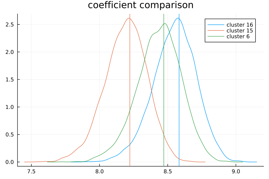
(Note that, in order to account for the base case, the OLS coefficients have been adjusted by adding the predicted intercept to their values.) Perhaps unsurprisingly, the modes of the densities predicted by Bayesian inference line up almost exactly with the coefficients from our classical linear model.
Future directions
As is often the case with statistics, this is a somewhat unsatisfying conclusion to our story: despite our best efforts, our Bayesian hierarchical model has failed to outperform the simplest imaginable baseline. But your journey needn’t end here—there are still a number of ways one could evolve this approach. For instance:
- The categorical home type variable (single-family residence / condo / townhouse) is also a suitable choice for a multilevel model.
- Our clusters may cover too broad a geographic area, or may be imperfect in other ways (e.g. shape): the Redfin dataset also provides a neighborhood label for more granularity, and a street address for an even finer-tuned segmentation.
- Past transactions on the same home may also be informative: pricing models frequently take into account the price history of an asset, if available (this was not available in the current dataset, though).
In any event, my goal with this post wasn’t to develop a perfect house pricing model (so, uh, mission accomplished?), but rather to explore both classical and Bayesian methods for addressing the challenges inherent in pricing homes. And arguably our main tool, Julia, has excelled at this: we were able to handle data manipulation and cleaning in an intuitive way from start to finish, plus work with a probablistic programming framework (Turing) from within the language itself. Speaking personally, Julia has largely replaced R as my statistical analysis tool of choice—and who knows, as packages like Flux.jl mature, maybe it will replace Python as well!